API Quickstart
Working example notebooks are available in the example folder.
Propensity Score
Propensity Score Estimation
from causalml.propensity import ElasticNetPropensityModel

pm = ElasticNetPropensityModel(n_fold=5, random_state=42)
ps = pm.fit_predict(X, y)
Propensity Score Matching
from causalml.match import NearestNeighborMatch, create_table_one

psm = NearestNeighborMatch(replace=False,
                           ratio=1,
                           random_state=42)
matched = psm.match_by_group(data=df,
                             treatment_col=treatment_col,
                             score_cols=score_cols,
                             groupby_col=groupby_col)

create_table_one(data=matched,
                 treatment_col=treatment_col,
                 features=covariates)
Average Treatment Effect (ATE) Estimation
Meta-learners and Uplift Trees
In addition to the Methodology section, you can find examples in the links below for Meta-Learner Algorithms and Tree-Based Algorithms
Meta-learners (S/T/X/R): meta_learners_with_synthetic_data.ipynb
Meta-learners (S/T/X/R) with multiple treatment: meta_learners_with_synthetic_data_multiple_treatment.ipynb
Comparing meta-learners across simulation setups: benchmark_simulation_studies.ipynb
Doubly Robust (DR) learner: dr_learner_with_synthetic_data.ipynb
TMLE learner: validation_with_tmle.ipynb
Uplift Trees: uplift_trees_with_synthetic_data.ipynb
from causalml.inference.meta import LRSRegressor
from causalml.inference.meta import XGBTRegressor, MLPTRegressor
from causalml.inference.meta import BaseXRegressor
from causalml.inference.meta import BaseRRegressor
from xgboost import XGBRegressor
from causalml.dataset import synthetic_data

y, X, treatment, _, _, e = synthetic_data(mode=1, n=1000, p=5, sigma=1.0)

lr = LRSRegressor()
te, lb, ub = lr.estimate_ate(X, treatment, y)
print('Average Treatment Effect (Linear Regression): {:.2f} ({:.2f}, {:.2f})'.format(te[0], lb[0], ub[0]))

xg = XGBTRegressor(random_state=42)
te, lb, ub = xg.estimate_ate(X, treatment, y)
print('Average Treatment Effect (XGBoost): {:.2f} ({:.2f}, {:.2f})'.format(te[0], lb[0], ub[0]))

nn = MLPTRegressor(hidden_layer_sizes=(10, 10),
                 learning_rate_init=.1,
                 early_stopping=True,
                 random_state=42)
te, lb, ub = nn.estimate_ate(X, treatment, y)
print('Average Treatment Effect (Neural Network (MLP)): {:.2f} ({:.2f}, {:.2f})'.format(te[0], lb[0], ub[0]))

xl = BaseXRegressor(learner=XGBRegressor(random_state=42))
te, lb, ub = xl.estimate_ate(X, treatment, y, e)
print('Average Treatment Effect (BaseXRegressor using XGBoost): {:.2f} ({:.2f}, {:.2f})'.format(te[0], lb[0], ub[0]))

rl = BaseRRegressor(learner=XGBRegressor(random_state=42))
te, lb, ub =  rl.estimate_ate(X=X, p=e, treatment=treatment, y=y)
print('Average Treatment Effect (BaseRRegressor using XGBoost): {:.2f} ({:.2f}, {:.2f})'.format(te[0], lb[0], ub[0]))
More algorithms
Treatment optimization algorithms
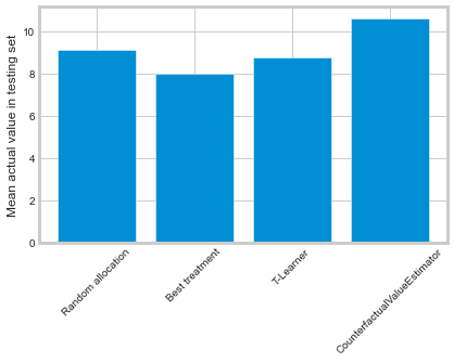
We have developed Counterfactual Unit Selection and Counterfactual Value Estimator methods, please find the code snippet below and details in the following notebooks:
from causalml.optimize import CounterfactualValueEstimator
from causalml.optimize import get_treatment_costs, get_actual_value

# load data set and train test split
df_train, df_test = train_test_split(df)
train_idx = df_train.index
test_idx = df_test.index
# some more code here to initiate and train the Model, and produce tm_pred
# please refer to the counterfactual_value_optimization notebook for complete example

# run the counterfactual calculation with TwoModel prediction
cve = CounterfactualValueEstimator(treatment=df_test['treatment_group_key'],
                                   control_name='control',
                                   treatment_names=conditions[1:],
                                   y_proba=y_proba,
                                   cate=tm_pred,
                                   value=conversion_value_array[test_idx],
                                   conversion_cost=cc_array[test_idx],
                                   impression_cost=ic_array[test_idx])

cve_best_idx = cve.predict_best()
cve_best = [conditions[idx] for idx in cve_best_idx]
actual_is_cve_best = df.loc[test_idx, 'treatment_group_key'] == cve_best
cve_value = actual_value.loc[test_idx][actual_is_cve_best].mean()

labels = [
    'Random allocation',
    'Best treatment',
    'T-Learner',
    'CounterfactualValueEstimator'
]
values  = [
    random_allocation_value,
    best_ate_value,
    tm_value,
    cve_value
]
# plot the result
plt.bar(labels, values)
Instrumental variables algorithms
2-Stage Least Squares (2SLS): iv_nlsym_synthetic_data.ipynb
Neural network based algorithms
CEVAE: cevae_example.ipynb
DragonNet: dragonnet_example.ipynb
Interpretation
Please see Interpretable Causal ML section
Validation
Please see Validation section
Synthetic Data Generation Process
Single Simulation
from causalml.dataset import *
# Generate synthetic data for single simulation
y, X, treatment, tau, b, e = synthetic_data(mode=1)
y, X, treatment, tau, b, e = simulate_nuisance_and_easy_treatment()
# Generate predictions for single simulation
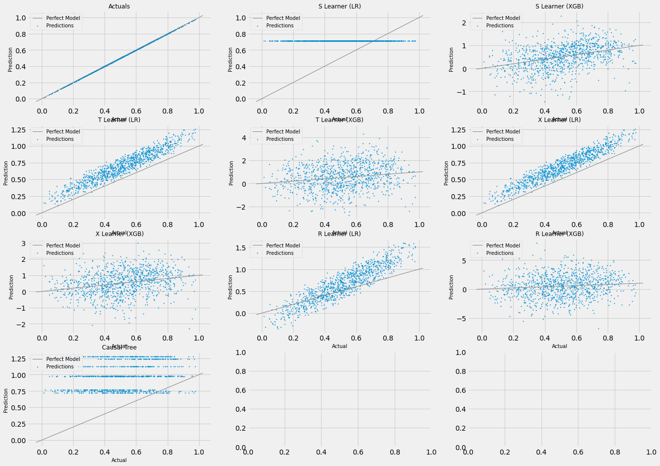
single_sim_preds = get_synthetic_preds(simulate_nuisance_and_easy_treatment, n=1000)
# Generate multiple scatter plots to compare learner performance for a single simulation
scatter_plot_single_sim(single_sim_preds)
# Visualize distribution of learner predictions for a single simulation
distr_plot_single_sim(single_sim_preds, kind='kde')
Multiple Simulations
from causalml.dataset import *
# Generalize performance summary over k simulations
num_simulations = 12
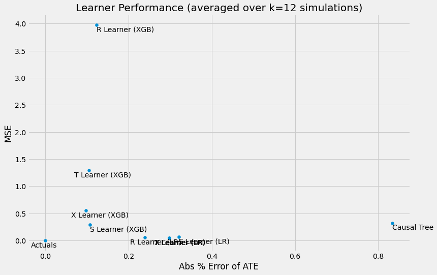
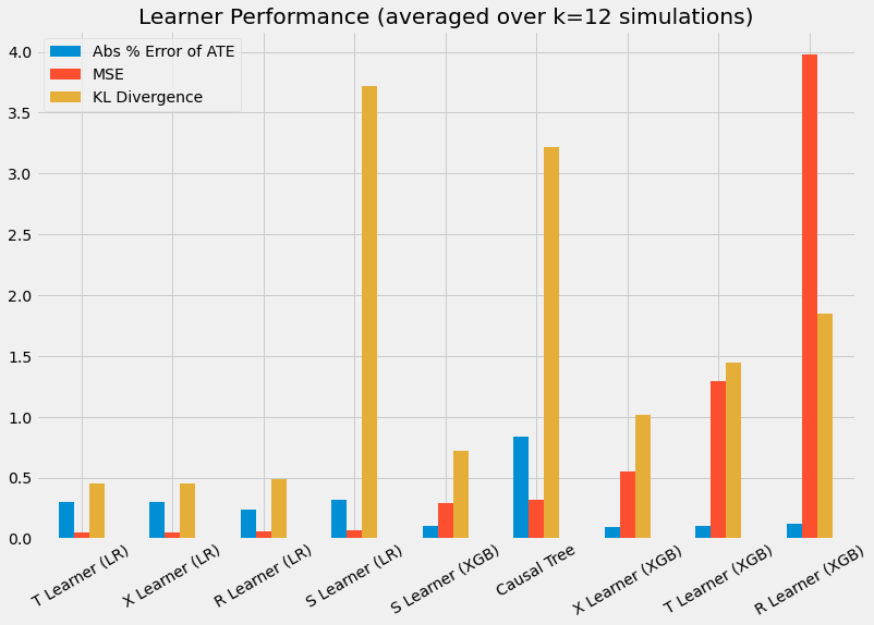
preds_summary = get_synthetic_summary(simulate_nuisance_and_easy_treatment, n=1000, k=num_simulations)
# Generate scatter plot of performance summary
scatter_plot_summary(preds_summary, k=num_simulations)
# Generate bar plot of performance summary
bar_plot_summary(preds_summary, k=num_simulations)
Sensitivity Analysis
For more details, please refer to the sensitivity_example_with_synthetic_data.ipynb notebook.
from causalml.metrics.sensitivity import Sensitivity
from causalml.metrics.sensitivity import SensitivitySelectionBias
from causalml.inference.meta import BaseXLearner
from sklearn.linear_model import LinearRegression

# Calling the Base XLearner class and return the sensitivity analysis summary report
learner_x = BaseXLearner(LinearRegression())
sens_x = Sensitivity(df=df, inference_features=INFERENCE_FEATURES, p_col='pihat',
                     treatment_col=TREATMENT_COL, outcome_col=OUTCOME_COL, learner=learner_x)
# Here for Selection Bias method will use default one-sided confounding function and alpha (quantile range of outcome values) input
sens_sumary_x = sens_x.sensitivity_analysis(methods=['Placebo Treatment',
                                                     'Random Cause',
                                                     'Subset Data',
                                                     'Random Replace',
                                                     'Selection Bias'], sample_size=0.5)

# Selection Bias: Alignment confounding Function
sens_x_bias_alignment = SensitivitySelectionBias(df, INFERENCE_FEATURES, p_col='pihat', treatment_col=TREATMENT_COL,
                                             outcome_col=OUTCOME_COL, learner=learner_x, confound='alignment',
                                             alpha_range=None)
# Plot the results by rsquare with partial r-square results by each individual features
sens_x_bias_alignment.plot(lls_x_bias_alignment, partial_rsqs_x_bias_alignment, type='r.squared', partial_rsqs=True)
Feature Selection
For more details, please refer to the feature_selection.ipynb notebook and the associated paper reference by Zhao, Zhenyu, et al.
from causalml.feature_selection.filters import FilterSelect
from causalml.dataset import make_uplift_classification

# define parameters for simulation
y_name = 'conversion'
treatment_group_keys = ['control', 'treatment1']
n = 100000
n_classification_features = 50
n_classification_informative = 10
n_classification_repeated = 0
n_uplift_increase_dict = {'treatment1': 8}
n_uplift_decrease_dict = {'treatment1': 4}
delta_uplift_increase_dict = {'treatment1': 0.1}
delta_uplift_decrease_dict = {'treatment1': -0.1}

# make a synthetic uplift data set
random_seed = 20200808
df, X_names = make_uplift_classification(
    treatment_name=treatment_group_keys,
    y_name=y_name,
    n_samples=n,
    n_classification_features=n_classification_features,
    n_classification_informative=n_classification_informative,
    n_classification_repeated=n_classification_repeated,
    n_uplift_increase_dict=n_uplift_increase_dict,
    n_uplift_decrease_dict=n_uplift_decrease_dict,
    delta_uplift_increase_dict = delta_uplift_increase_dict,
    delta_uplift_decrease_dict = delta_uplift_decrease_dict,
    random_seed=random_seed
)

# Feature selection with Filter method
filter_f = FilterSelect()
method = 'F'
f_imp = filter_f.get_importance(df, X_names, y_name, method,
                      treatment_group = 'treatment1')
print(f_imp)

# Use likelihood ratio test method
method = 'LR'
lr_imp = filter_f.get_importance(df, X_names, y_name, method,
                      treatment_group = 'treatment1')
print(lr_imp)

# Use KL divergence method
method = 'KL'
kl_imp = filter_f.get_importance(df, X_names, y_name, method,
                      treatment_group = 'treatment1',
                      n_bins=10)
print(kl_imp)