Propensity Score Calibration

We use a toy example to demonstrate the calibration of propensity scores generated by a simple GaussianNB model.

Reproduce sci-kit learn example

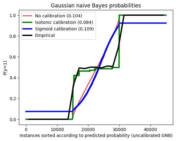
First, we reproduce a simple “three-blob” sci-kit learn example which illustrates how using a CalibratedClassifierCV improves propensity predictions under both “isotonic” and “sigmoid” methods.

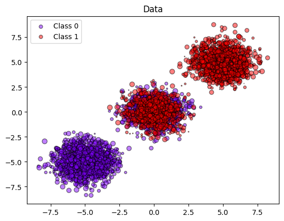
In this example, we fit a GaussianNB model to a population containing three blobs and essentially one predictive covariate (see graph):

• bottom left (all class 0, treatment propensity=0)

• middle (50/50 mix of purple and red, treatment propensity=0.5)

• top right (all class 1, treatment propensity=1)

We see that the isotonic calibration performs better than sigmoid calibration.

# Following example at:
# https://scikit-learn.org/stable/auto_examples/calibration/plot_calibration.html#sphx-glr-auto-examples-calibration-plot-calibration-py

import numpy as np

from sklearn.datasets import make_blobs
from sklearn.model_selection import train_test_split

n_samples = 50000

# Generate 3 blobs with 2 classes where the second blob contains
# half positive samples and half negative samples. Probability in this
# blob is therefore 0.5.
centers = [(-5, -5), (0, 0), (5, 5)]
X, y = make_blobs(n_samples=n_samples, centers=centers, shuffle=False, random_state=42)

y[: n_samples // 2] = 0
y[n_samples // 2 :] = 1
sample_weight = np.random.RandomState(42).rand(y.shape[0])

# split train, test for calibration
X_train, X_test, y_train, y_test, sw_train, sw_test = train_test_split(
    X, y, sample_weight, test_size=0.9, random_state=42
)

from sklearn.calibration import CalibratedClassifierCV
from sklearn.metrics import brier_score_loss
from sklearn.naive_bayes import GaussianNB

# With no calibration
clf = GaussianNB()
clf.fit(X_train, y_train)  # GaussianNB itself does not support sample-weights
prob_pos_clf = clf.predict_proba(X_test)[:, 1]

# With isotonic calibration
clf_isotonic = CalibratedClassifierCV(clf, cv=2, method="isotonic")
clf_isotonic.fit(X_train, y_train, sample_weight=sw_train)
prob_pos_isotonic = clf_isotonic.predict_proba(X_test)[:, 1]

# With sigmoid calibration
clf_sigmoid = CalibratedClassifierCV(clf, cv=2, method="sigmoid")
clf_sigmoid.fit(X_train, y_train, sample_weight=sw_train)
prob_pos_sigmoid = clf_sigmoid.predict_proba(X_test)[:, 1]

print("Brier score losses: (the smaller the better)")

clf_score = brier_score_loss(y_test, prob_pos_clf, sample_weight=sw_test)
print("No calibration: %1.3f" % clf_score)

clf_isotonic_score = brier_score_loss(y_test, prob_pos_isotonic, sample_weight=sw_test)
print("With isotonic calibration: %1.3f" % clf_isotonic_score)

clf_sigmoid_score = brier_score_loss(y_test, prob_pos_sigmoid, sample_weight=sw_test)
print("With sigmoid calibration: %1.3f" % clf_sigmoid_score)

Brier score losses: (the smaller the better)
No calibration: 0.104
With isotonic calibration: 0.084
With sigmoid calibration: 0.109

import matplotlib.pyplot as plt
from matplotlib import cm

plt.figure()
y_unique = np.unique(y)
colors = cm.rainbow(np.linspace(0.0, 1.0, y_unique.size))
for this_y, color in zip(y_unique, colors):
    this_X = X_train[y_train == this_y]
    this_sw = sw_train[y_train == this_y]
    plt.scatter(
        this_X[:, 0],
        this_X[:, 1],
        s=this_sw * 50,
        c=color[np.newaxis, :],
        alpha=0.5,
        edgecolor="k",
        label="Class %s" % this_y,
    )
plt.legend(loc="best")
plt.title("Data")

plt.figure()

order = np.lexsort((prob_pos_clf,))
plt.plot(prob_pos_clf[order], "r", label="No calibration (%1.3f)" % clf_score)
plt.plot(
    prob_pos_isotonic[order],
    "g",
    linewidth=3,
    label="Isotonic calibration (%1.3f)" % clf_isotonic_score,
)
plt.plot(
    prob_pos_sigmoid[order],
    "b",
    linewidth=3,
    label="Sigmoid calibration (%1.3f)" % clf_sigmoid_score,
)
plt.plot(
    np.linspace(0, y_test.size, 51)[1::2],
    y_test[order].reshape(25, -1).mean(1),
    "k",
    linewidth=3,
    label=r"Empirical",
)
plt.ylim([-0.05, 1.05])
plt.xlabel("Instances sorted according to predicted probability (uncalibrated GNB)")
plt.ylabel("P(y=1)")
plt.legend(loc="upper left")
plt.title("Gaussian naive Bayes probabilities")

plt.show()

Modify above example to use IsotonicRegression

We now work through the above example using IsotonicRegression and without CalibratedClassifierCV. To use calibrate with IsotonicRegression, we follow the framework implemented in CausalML’s propensity.py and define two functions calibrate_iso(...) and compute_propensity_score(...).

import logging
from sklearn.isotonic import IsotonicRegression

import matplotlib.pyplot as plt
import seaborn as sns
import numpy as np
import pandas as pd

%matplotlib inline

from causalml.propensity import (
    ElasticNetPropensityModel,
    GradientBoostedPropensityModel,
    LogisticRegressionPropensityModel,
)

def calibrate_iso(ps, treatment):
    """Calibrate propensity scores with IsotonicRegression.

    Ref: https://scikit-learn.org/stable/modules/isotonic.html

    Args:
        ps (numpy.array): a propensity score vector
        treatment (numpy.array): a binary treatment vector (0: control, 1: treated)

    Returns:
        (numpy.array): a calibrated propensity score vector
    """

    print("calibrate_iso")
    two_eps = 2.0 * np.finfo(float).eps
    pm_ir = IsotonicRegression(out_of_bounds="clip", y_min=two_eps, y_max=1.0 - two_eps)
    ps_ir = pm_ir.fit_transform(ps, treatment)

    return ps_ir


def compute_propensity_score(
    X, treatment, p_model=None, X_pred=None, treatment_pred=None, calibrate_p="iso"
):
    """Generate propensity score if user didn't provide

    Args:
        X (np.matrix): features for training
        treatment (np.array or pd.Series): a treatment vector for training
        p_model (propensity model object, optional):
            ElasticNetPropensityModel (default) / GradientBoostedPropensityModel
        X_pred (np.matrix, optional): features for prediction
        treatment_pred (np.array or pd.Series, optional): a treatment vector for prediciton
        calibrate_p (bool, optional): whether calibrate the propensity score

    Returns:
        (tuple)
            - p (numpy.ndarray): propensity score
            - p_model (PropensityModel): a trained PropensityModel object
    """

    print("using local compute_propensity_score")

    if treatment_pred is None:
        treatment_pred = treatment.copy()
    if p_model is None:
        p_model = ElasticNetPropensityModel()

    p_model.fit(X, treatment)

    if X_pred is None:
        try:
            p = p_model.predict_proba(X)[:, 1]
        except AttributeError:
            print("predict_proba not available, using predict instead")
            p = p_model.predict(X)
    else:
        try:
            p = p_model.predict_proba(X_pred)[:, 1]
        except AttributeError:
            print("predict_proba not available, using predict instead")
            p = p_model.predict(X_pred)

    if calibrate_p == "iso":
        print("Isotonic calibrating propensity scores only.  Returning model=None.")
        p = calibrate_iso(p, treatment_pred)
        p_model = None
    elif calibrate_p == "pygam":
        print("pyGAM calibrating propensity scores only.  Returning model=None.")
        p = calibrate_pygam(p, treatment_pred)
        p_model = None

    # force the p values within the range
    eps = np.finfo(float).eps
    p = np.where(p < 0 + eps, 0 + eps * 1.001, p)
    p = np.where(p > 1 - eps, 1 - eps * 1.001, p)

    return p, p_model

Calculate the uncalibrated propensity scores

# Without calibration, naive Bayes
cml_prob_pos_uc, psm_cps_uc = compute_propensity_score(X_train, y_train, p_model=clf, X_pred=X_test, calibrate_p=False)

using local compute_propensity_score

# With isotonic calibration
cml_prob_pos_cal_iso, psm_cps_cal_iso = compute_propensity_score(X_train, y_train, p_model=clf, X_pred=X_test, treatment_pred=y_test, calibrate_p="iso")

using local compute_propensity_score
Isotonic calibrating propensity scores only.  Returning model=None.
calibrate_iso

print("Brier score losses: (the smaller the better)")

cml_uc_score = brier_score_loss(y_test, cml_prob_pos_uc)
print("No calibration: %1.3f" % cml_uc_score)

cml_cal_iso_score = brier_score_loss(y_test, cml_prob_pos_cal_iso)
print("With isotonic calibration: %1.3f" % cml_cal_iso_score)

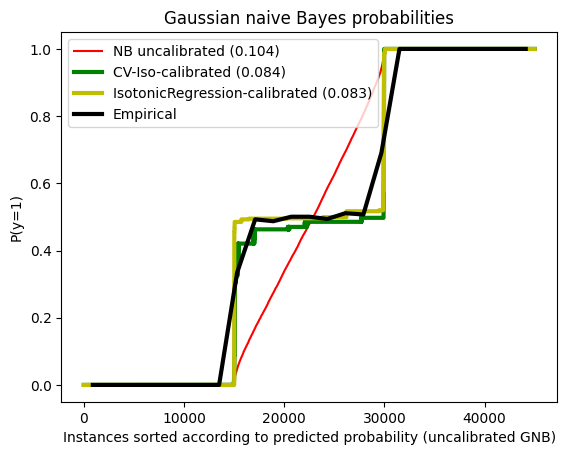
Brier score losses: (the smaller the better)
No calibration: 0.104
With isotonic calibration: 0.083

Plot result

We confirm that using the CausalML calibration method using IsotonicRegression performs similarly to the CalibratedClassifierCV method in the original example, and that both match the empircal distribution better than the uncalibrated Naïve Bayes scores.

import matplotlib.pyplot as plt
from matplotlib import cm

plt.figure()
y_unique = np.unique(y)
colors = cm.rainbow(np.linspace(0.0, 1.0, y_unique.size))
for this_y, color in zip(y_unique, colors):
    this_X = X_train[y_train == this_y]
    this_sw = sw_train[y_train == this_y]
    plt.scatter(
        this_X[:, 0],
        this_X[:, 1],
        s=this_sw * 50,
        c=color[np.newaxis, :],
        alpha=0.5,
        edgecolor="k",
        label="Class %s" % this_y,
    )
plt.legend(loc="best")
plt.title("Data")

plt.figure()

order = np.lexsort((prob_pos_clf,))
# plt.plot(prob_pos_clf[order], "r", label="No calibration (%1.3f)" % clf_score)
plt.plot(
    cml_prob_pos_uc[order],
    "r",
    # linewidth=3,
    # linestyle="--",
    label="NB uncalibrated (%1.3f)" % cml_uc_score,
)
plt.plot(
    prob_pos_isotonic[order],
    "g",
    linewidth=3,
    label="CV-Iso-calibrated (%1.3f)" % clf_isotonic_score,
)
plt.plot(
    cml_prob_pos_cal_iso[order],
    "y",
    linewidth=3,
    linestyle="-",
    label="IsotonicRegression-calibrated (%1.3f)" % cml_cal_iso_score,
)
plt.plot(
    np.linspace(0, y_test.size, 51)[1::2],
    y_test[order].reshape(25, -1).mean(1),
    "k",
    linewidth=3,
    label=r"Empirical",
)
plt.ylim([-0.05, 1.05])
plt.xlabel("Instances sorted according to predicted probability (uncalibrated GNB)")
plt.ylabel("P(y=1)")
plt.legend(loc="upper left")
plt.title("Gaussian naive Bayes probabilities")

plt.show()