Causal Trees/Forests Interpretation with Feature Importance and SHAP Values
[1]:
%reload_ext autoreload
%autoreload 2
%matplotlib inline
[1]:
import pandas as pd
import numpy as np
import multiprocessing as mp

np.random.seed(42)

from sklearn.model_selection import train_test_split
from sklearn.inspection import permutation_importance

# Currently causalml shap support is experimental and is available by installing from source
# PR: https://github.com/shap/shap/pull/3273
import shap

import causalml
from causalml.metrics import plot_gain, plot_qini, qini_score
from causalml.dataset import synthetic_data
from causalml.inference.tree import plot_dist_tree_leaves_values, get_tree_leaves_mask
from causalml.inference.tree import CausalRandomForestRegressor, CausalTreeRegressor
from causalml.inference.tree.utils import timeit

import matplotlib.pyplot as plt
import seaborn as sns

%config InlineBackend.figure_format = 'retina'
Failed to import duecredit due to No module named 'duecredit'
[2]:
import importlib
for libname in ["causalml", "shap"]:
    print(f"{libname}: {importlib.metadata.version(libname)}")
causalml: 0.15.5
shap: 0.48.0
[3]:
# Simulate randomized trial: mode=2
y, X, w, tau, b, e = synthetic_data(mode=2, n=2000, p=10, sigma=3.0)

df = pd.DataFrame(X)
feature_names = [f'feature_{i}' for i in range(X.shape[1])]
df.columns = feature_names
df['outcome'] = y
df['treatment'] = w
df['treatment_effect'] = tau
[4]:
# Split data to training and testing samples for model validation
df_train, df_test = train_test_split(df, test_size=0.2, random_state=111)
n_train, n_test = df_train.shape[0], df_test.shape[0]

X_train, y_train = df_train[feature_names], df_train['outcome'].values
X_test, y_test = df_test[feature_names], df_test['outcome'].values
treatment_train, treatment_test = df_train['treatment'].values, df_test['treatment'].values
effect_test = df_test['treatment_effect'].values

observation = X_test.loc[[0]]
CausalTreeRegressor
[5]:
ctree = CausalTreeRegressor()
ctree.fit(X=X_train.values, y=y_train, treatment=treatment_train)
[5]:
CausalTreeRegressor()In a Jupyter environment, please rerun this cell to show the HTML representation or trust the notebook.
On GitHub, the HTML representation is unable to render, please try loading this page with nbviewer.org.
Parameters
| criterion | 'causal_mse' | |
| splitter | 'best' | |
| alpha | 0.05 | |
| control_name | 0 | |
| max_depth | None | |
| min_samples_split | 60 | |
| min_weight_fraction_leaf | 0.0 | |
| max_features | None | |
| max_leaf_nodes | None | |
| min_impurity_decrease | -inf | |
| ccp_alpha | 0.0 | |
| groups_penalty | 0.5 | |
| min_group_size | 50 | |
| min_samples_leaf | 100 | |
| random_state | None | |
| groups_cnt | False | |
| groups_cnt_mode | 'nodes' |
CausalRandomForestRegressor
[6]:
crforest = CausalRandomForestRegressor(criterion="causal_mse",
                                  min_samples_leaf=200,
                                  control_name=0,
                                  n_estimators=50,
                                  n_jobs=mp.cpu_count() - 1)
crforest.fit(X=X_train, y=y_train, treatment=treatment_train)
[6]:
CausalRandomForestRegressor(min_samples_leaf=200, n_estimators=50, n_jobs=11)In a Jupyter environment, please rerun this cell to show the HTML representation or trust the notebook.
On GitHub, the HTML representation is unable to render, please try loading this page with nbviewer.org.
Parameters
| n_estimators | 50 | |
| control_name | 0 | |
| criterion | 'causal_mse' | |
| alpha | 0.05 | |
| max_depth | None | |
| min_samples_split | 60 | |
| min_samples_leaf | 200 | |
| min_group_size | 50 | |
| min_weight_fraction_leaf | 0.0 | |
| max_features | 1.0 | |
| max_leaf_nodes | None | |
| min_impurity_decrease | -inf | |
| bootstrap | True | |
| oob_score | False | |
| n_jobs | 11 | |
| random_state | None | |
| verbose | 0 | |
| warm_start | False | |
| ccp_alpha | 0.0 | |
| groups_penalty | 0.5 | |
| max_samples | None | |
| groups_cnt | True | |
| groups_cnt_mode | 'nodes' |
1. Impurity-based feature importance
[7]:
df_importances = pd.DataFrame({'tree': ctree.feature_importances_,
                               'forest': crforest.feature_importances_,
                               'feature': feature_names
                              })
forest_std = np.std([tree.feature_importances_ for tree in crforest.estimators_], axis=0)

fig, ax = plt.subplots()
df_importances['tree'].plot.bar(ax=ax)
ax.set_title("Causal Tree feature importances")
ax.set_ylabel("Mean decrease in impurity")
ax.set_xticklabels(feature_names, rotation=45)
plt.show()

fig, ax = plt.subplots()
df_importances['forest'].plot.bar(yerr=forest_std, ax=ax)
ax.set_title("Causal Forest feature importances")
ax.set_ylabel("Mean decrease in impurity")
ax.set_xticklabels(feature_names, rotation=45)
plt.show()


2. Permutation-based feature importance
[8]:
for name, model in zip(('Causal Tree', 'Causal Forest'), (ctree, crforest)):

    imp = permutation_importance(model, X_test, y_test,
                                 n_repeats=50,
                                 random_state=0)

    fig, ax = plt.subplots()
    ax.set_title(f"{name} feature importances")
    ax.set_ylabel("Mean decrease in impurity")
    plt.bar(feature_names, imp['importances_mean'], yerr=imp['importances_std'])
    ax.set_xticklabels(feature_names, rotation=45)
    plt.show()


SHAP values
TreeExplainer
Details: https://shap.readthedocs.io/en/latest/generated/shap.TreeExplainer.html#shap.TreeExplainer
CausalTree
[10]:
tree_explainer = shap.TreeExplainer(ctree)
# Expected values for treatment=0 and treatment=1. i.e. Y|X,T=0 and Y|X,T=1
tree_explainer.expected_value
[10]:
array([0.93121212, 1.63459276])
[11]:
tree_explainer
[11]:
<shap.explainers._tree.TreeExplainer at 0x7ecc19419250>
[12]:
# (Y|X,T=0, Y|X,T=1,  [Y|X,T=1] - [Y|X,T=0])
ctree.predict(observation, with_outcomes=True)
[12]:
array([[ 2.3146749 , 2.03953544, -0.27513945]])
[13]:
observation
[13]:
| feature_0 | feature_1 | feature_2 | feature_3 | feature_4 | feature_5 | feature_6 | feature_7 | feature_8 | feature_9 | |
|---|---|---|---|---|---|---|---|---|---|---|
| 0 | 0.496714 | -0.138264 | 0.647689 | 1.52303 | -0.234153 | -0.234137 | 1.579213 | 0.767435 | -0.469474 | 0.54256 |
[14]:
# CausalTree
# Tree Explainer for treatment=0
shap.initjs()

treatment_idx = 0
shap_values = tree_explainer.shap_values(observation)
shap.force_plot(
    base_value=np.array([tree_explainer.expected_value[treatment_idx]]),
    shap_values=shap_values[:, :, treatment_idx],
    features=observation,
    matplotlib=True
)

[15]:
# CausalTree
# Tree Explainer for treatment=1
shap.initjs()

treatment_idx = 1
shap_values = tree_explainer.shap_values(observation)
shap.force_plot(
    base_value=np.array([tree_explainer.expected_value[treatment_idx]]),
    shap_values=shap_values[:, :, treatment_idx],
    features=observation,
    matplotlib=True
)

CausalRandomForest
[16]:
cforest_explainer = shap.TreeExplainer(crforest)
# Expected values for treatment=0 and treatment=1. i.e. Y|X,T=0 and Y|X,T=1
cforest_explainer.expected_value
[16]:
array([0.93203354, 1.61854881])
[17]:
# (Y|X,T=0, Y|X,T=1,  [Y|X,T=1] - [Y|X,T=0])
crforest.predict(observation, with_outcomes=True)
[17]:
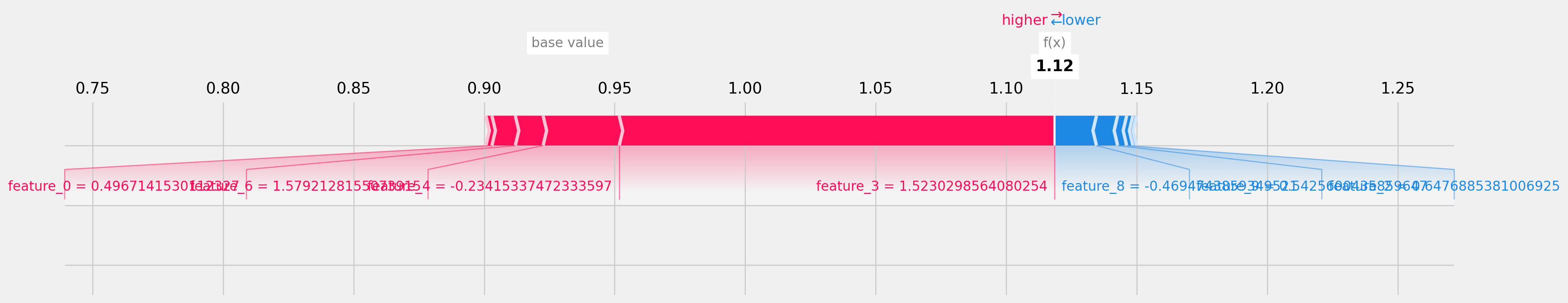
array([[1.11856369, 1.9490421 , 0.83047841]])
[18]:
# CausalRandomForest
# Tree Explainer for treatment=0
shap.initjs()

treatment_idx = 0
shap_values = cforest_explainer.shap_values(observation)

shap.force_plot(
    base_value=np.array([cforest_explainer.expected_value[treatment_idx]]),
    shap_values=shap_values[:, :, treatment_idx],
    features=observation,
    matplotlib=True
)
[19]:
# CausalRandomForest
# Tree Explainer for treatment=1
shap.initjs()

treatment_idx = 1
shap_values = cforest_explainer.shap_values(observation)

shap.force_plot(
    base_value=np.array([cforest_explainer.expected_value[treatment_idx]]),
    shap_values=shap_values[:, :, treatment_idx],
    features=observation,
    matplotlib=True
)

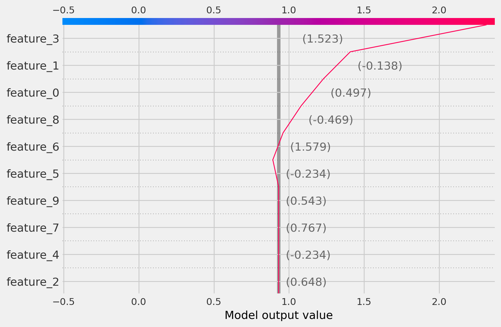
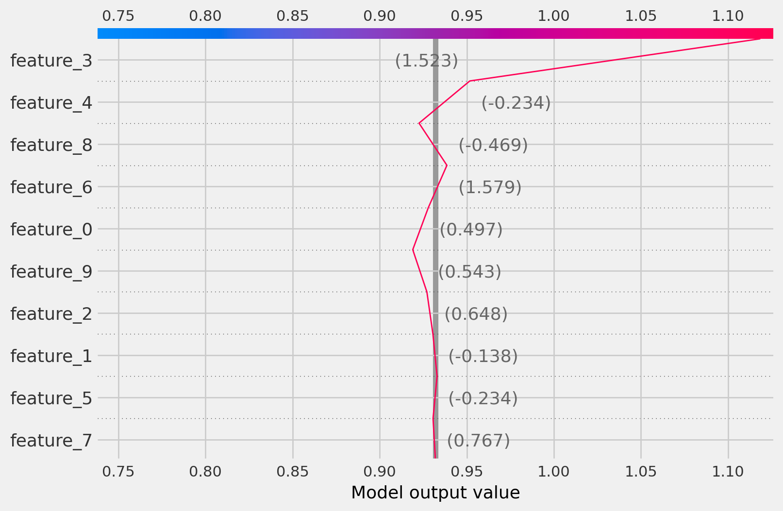
Decision plots
CausalTree
[20]:
treatment_idx=0
shap_values = tree_explainer.shap_values(observation)
shap.decision_plot(
    base_value=np.array([tree_explainer.expected_value[treatment_idx]]),
    shap_values=shap_values[:, :, treatment_idx],
    features=observation
)
treatment_idx=1
shap.decision_plot(
    base_value=np.array([tree_explainer.expected_value[treatment_idx]]),
    shap_values=shap_values[:, :, treatment_idx],
    features=observation
)
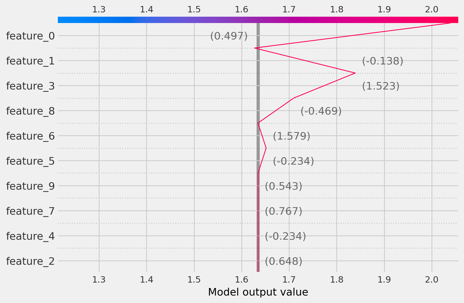
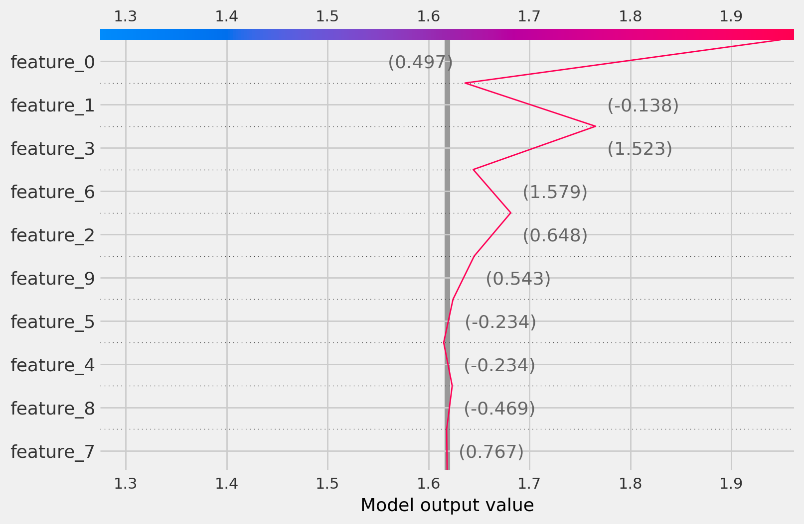
CausalRandomForest
[21]:
treatment_idx=0
shap_values = cforest_explainer.shap_values(observation)
shap.decision_plot(
    base_value=np.array([cforest_explainer.expected_value[treatment_idx]]),
    shap_values=shap_values[:, :, treatment_idx],
    features=observation
)
treatment_idx=1
shap.decision_plot(
    base_value=np.array([cforest_explainer.expected_value[treatment_idx]]),
    shap_values=shap_values[:, :, treatment_idx],
    features=observation
)
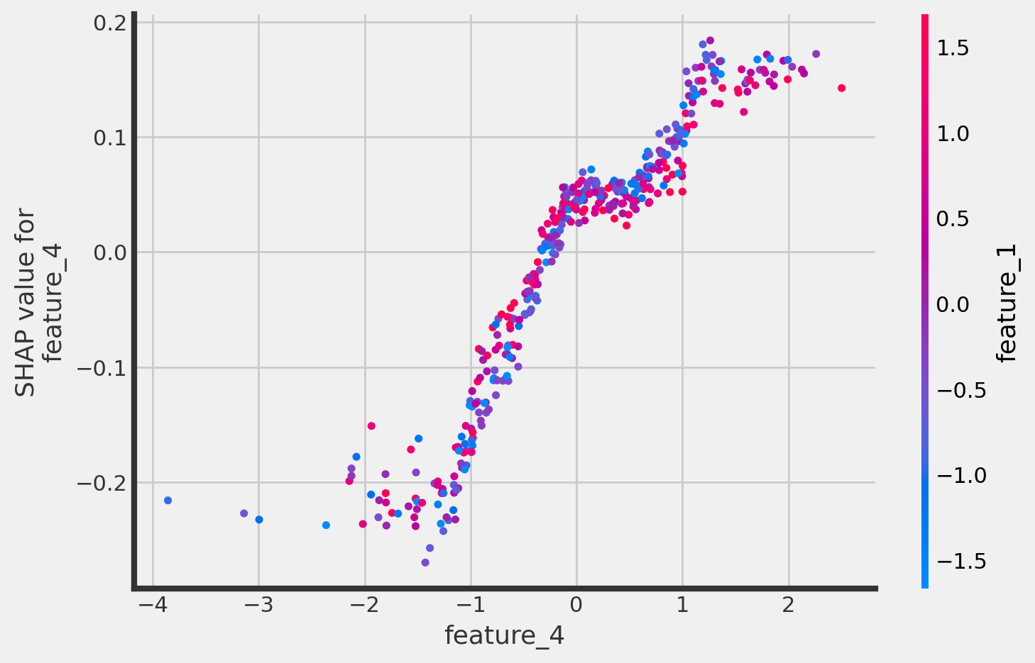
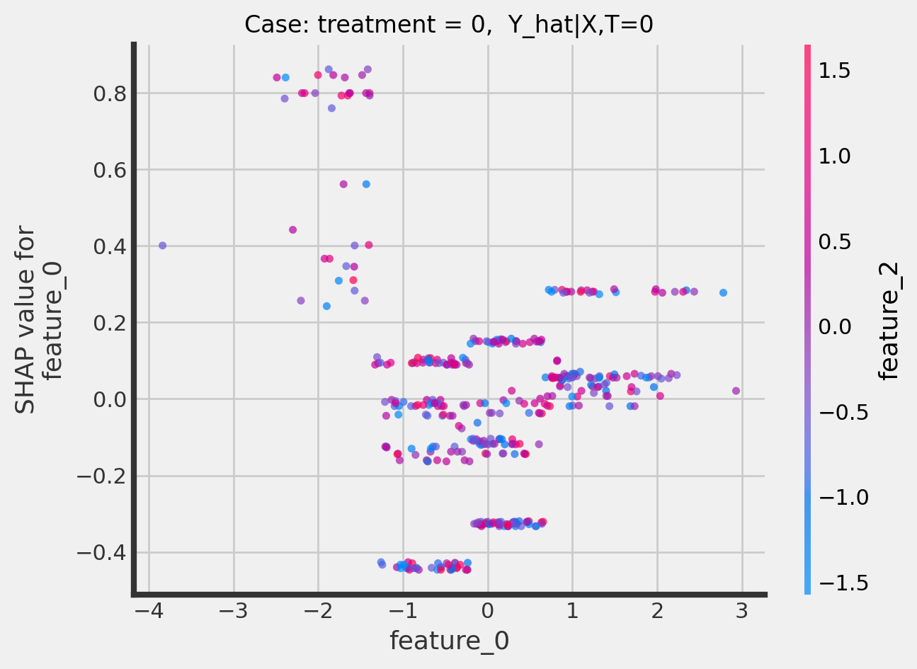
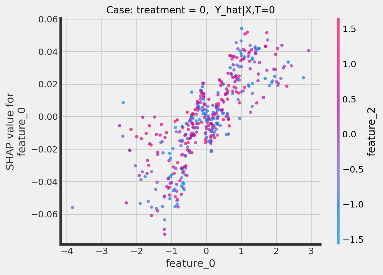
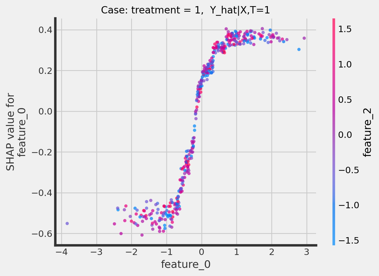
Dependence plots
CausalTree
[22]:
treatment_indices = [0, 1]
for i in treatment_indices:
    fig, ax = plt.subplots()
    ax.set_title(f"Case: treatment = {i},  Y_hat|X,T={i}", fontsize=12)
    shap.dependence_plot(
        "feature_0",
        tree_explainer.shap_values(X_test)[:, :, i],
        X_test,
        interaction_index="feature_2",
        alpha=0.7,
        ax=ax
    )
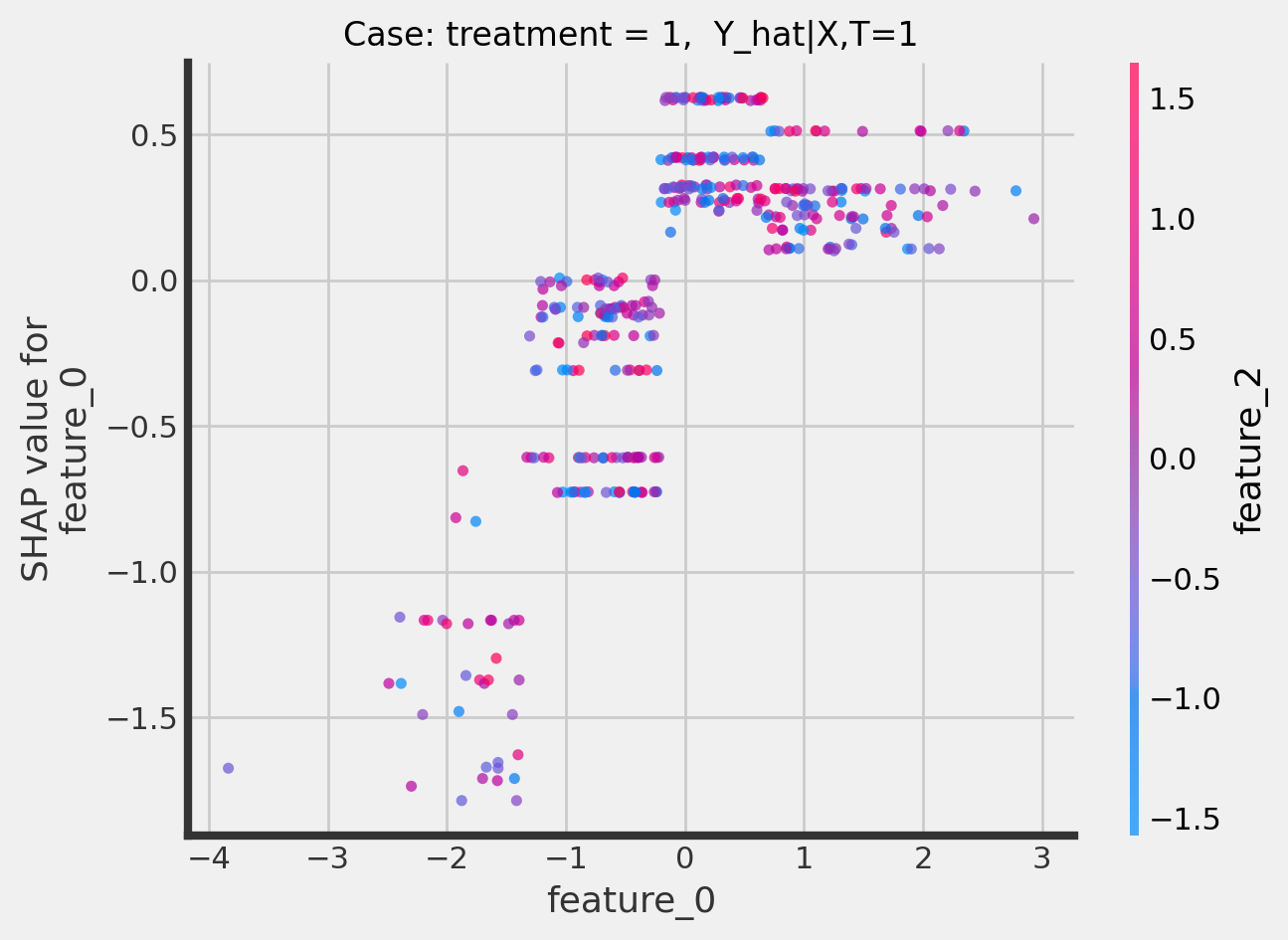
CausalRandomForest
[23]:
treatment_indices = [0, 1]
for i in treatment_indices:
    fig, ax = plt.subplots()
    ax.set_title(f"Case: treatment = {i},  Y_hat|X,T={i}", fontsize=12)
    shap.dependence_plot(
        "feature_0",
        cforest_explainer.shap_values(X_test)[:, :, i],
        X_test,
        interaction_index="feature_2",
        alpha=0.7,
        ax=ax
    )
[ ]: