Uplift Curves with TMLE Example
This notebook demonstrates the issue of using uplift curves without knowing true treatment effect and how to solve it by using TMLE as a proxy of the true treatment effect.
[1]:
%reload_ext autoreload
%autoreload 2
%matplotlib inline
[2]:
import os
base_path = os.path.abspath("../")
os.chdir(base_path)
[3]:
import logging
from matplotlib import pyplot as plt
import numpy as np
import pandas as pd
from sklearn.model_selection import train_test_split, KFold
import sys
import warnings
warnings.simplefilter("ignore", UserWarning)

from lightgbm import LGBMRegressor
[4]:
import causalml

from causalml.dataset import synthetic_data
from causalml.inference.meta import BaseXRegressor, TMLELearner
from causalml.metrics.visualize import *

import importlib
print(importlib.metadata.version('causalml') )
/Users/jeong/dev/causalml/.venv/lib/python3.12/site-packages/tqdm/auto.py:21: TqdmWarning: IProgress not found. Please update jupyter and ipywidgets. See https://ipywidgets.readthedocs.io/en/stable/user_install.html
  from .autonotebook import tqdm as notebook_tqdm
Failed to import duecredit due to No module named 'duecredit'
0.15.5.dev0
[5]:
logger = logging.getLogger('causalml')
logger.setLevel(logging.DEBUG)
plt.style.use('fivethirtyeight')
Generating Synthetic Data
[6]:
# Generate synthetic data using mode 1
y, X, treatment, tau, b, e = synthetic_data(mode=1, n=1000000, p=10, sigma=5.)
[7]:
X_train, X_test, y_train, y_test, e_train, e_test, treatment_train, treatment_test, tau_train, tau_test, b_train, b_test = train_test_split(X, y, e, treatment, tau, b, test_size=0.5, random_state=42)
Calculating Individual Treatment Effect (ITE/CATE)
[8]:
# X Learner
learner_x = BaseXRegressor(learner=LGBMRegressor())
learner_x.fit(X=X_train, treatment=treatment_train, y=y_train)
cate_x_test = learner_x.predict(X=X_test, p=e_test, treatment=treatment_test).flatten()
[LightGBM] [Info] Auto-choosing row-wise multi-threading, the overhead of testing was 0.001193 seconds.
You can set `force_row_wise=true` to remove the overhead.
And if memory is not enough, you can set `force_col_wise=true`.
[LightGBM] [Info] Total Bins 2550
[LightGBM] [Info] Number of data points in the train set: 240810, number of used features: 10
[LightGBM] [Info] Start training from score 1.031908
[LightGBM] [Info] Auto-choosing row-wise multi-threading, the overhead of testing was 0.000924 seconds.
You can set `force_row_wise=true` to remove the overhead.
And if memory is not enough, you can set `force_col_wise=true`.
[LightGBM] [Info] Total Bins 2550
[LightGBM] [Info] Number of data points in the train set: 259190, number of used features: 10
[LightGBM] [Info] Start training from score 1.918515
[LightGBM] [Info] Auto-choosing row-wise multi-threading, the overhead of testing was 0.001063 seconds.
You can set `force_row_wise=true` to remove the overhead.
And if memory is not enough, you can set `force_col_wise=true`.
[LightGBM] [Info] Total Bins 2550
[LightGBM] [Info] Number of data points in the train set: 240810, number of used features: 10
[LightGBM] [Info] Start training from score 0.374437
[LightGBM] [Info] Auto-choosing row-wise multi-threading, the overhead of testing was 0.000885 seconds.
You can set `force_row_wise=true` to remove the overhead.
And if memory is not enough, you can set `force_col_wise=true`.
[LightGBM] [Info] Total Bins 2550
[LightGBM] [Info] Number of data points in the train set: 259190, number of used features: 10
[LightGBM] [Info] Start training from score 0.624147
[9]:
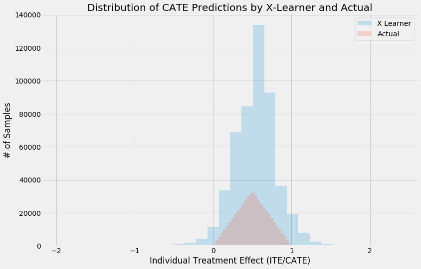
alpha=0.2
bins=30
plt.figure(figsize=(12,8))
plt.hist(cate_x_test, alpha=alpha, bins=bins, label='X Learner')
plt.hist(tau_test, alpha=alpha, bins=bins, label='Actual')

plt.title('Distribution of CATE Predictions by X-Learner and Actual')
plt.xlabel('Individual Treatment Effect (ITE/CATE)')
plt.ylabel('# of Samples')
_=plt.legend()
Validating CATE without TMLE
[10]:
df = pd.DataFrame({'y': y_test, 'w': treatment_test, 'tau': tau_test, 'X-Learner': cate_x_test, 'Actual': tau_test})
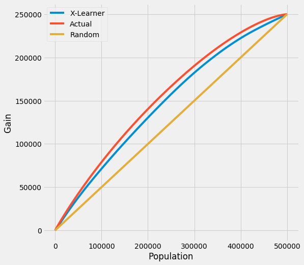
Uplift Curve With Ground Truth
If true treatment effect is known as in simulations, the uplift curve of a model uses the cumulative sum of the treatment effect sorted by model’s CATE estimate.
In the figure below, the uplift curve of X-learner shows positive lift close to the optimal lift by the ground truth.
[11]:
plot(df, outcome_col='y', treatment_col='w', treatment_effect_col='tau')
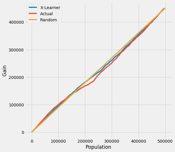
Uplift Curve Without Ground Truth
If true treatment effect is unknown as in practice, the uplift curve of a model uses the cumulative mean difference of outcome in the treatment and control group sorted by model’s CATE estimate.
In the figure below, the uplift curves of X-learner as well as the ground truth show no lift incorrectly.
[12]:
plot(df.drop('tau', axis=1), outcome_col='y', treatment_col='w')
TMLE
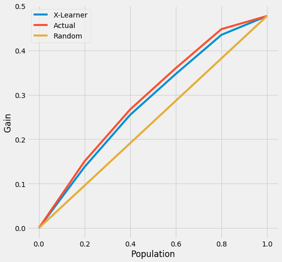
Uplift Curve with TMLE as Ground Truth
By using TMLE as a proxy of the ground truth, the uplift curves of X-learner and the ground truth become close to the original using the ground truth.
[13]:
n_fold = 5
kf = KFold(n_splits=n_fold)
[14]:
df = pd.DataFrame({'y': y_test, 'w': treatment_test, 'p': e_test, 'X-Learner': cate_x_test, 'Actual': tau_test})
[15]:
inference_cols = []
for i in range(X_test.shape[1]):
    col = 'col_' + str(i)
    df[col] = X_test[:,i]
    inference_cols.append(col)
[16]:
df.head()
[16]:
| y | w | p | X-Learner | Actual | col_0 | col_1 | col_2 | col_3 | col_4 | col_5 | col_6 | col_7 | col_8 | col_9 | |
|---|---|---|---|---|---|---|---|---|---|---|---|---|---|---|---|
| 0 | -1.172418 | 0 | 0.306314 | 0.292809 | 0.369913 | 0.564180 | 0.175646 | 0.811024 | 0.347398 | 0.873862 | 0.822687 | 0.615974 | 0.178150 | 0.320590 | 0.384264 |
| 1 | 0.289621 | 0 | 0.290396 | 0.296887 | 0.424024 | 0.717296 | 0.130751 | 0.927909 | 0.453772 | 0.300610 | 0.561574 | 0.599298 | 0.537041 | 0.616589 | 0.444704 |
| 2 | -3.709188 | 1 | 0.873150 | 0.737726 | 0.595008 | 0.468088 | 0.721929 | 0.174398 | 0.190066 | 0.519165 | 0.880392 | 0.868682 | 0.606476 | 0.585635 | 0.697090 |
| 3 | 2.556804 | 1 | 0.900000 | 0.292399 | 0.711302 | 0.713268 | 0.709336 | 0.880897 | 0.246433 | 0.574616 | 0.004385 | 0.897898 | 0.122412 | 0.691561 | 0.089741 |
| 4 | 5.151192 | 1 | 0.761681 | 0.569939 | 0.854140 | 0.782163 | 0.926117 | 0.697098 | 0.133041 | 0.153903 | 0.190420 | 0.943172 | 0.004570 | 0.607202 | 0.386699 |
[17]:
tmle_df = get_tmlegain(df, inference_col=inference_cols, outcome_col='y', treatment_col='w', p_col='p',
                       n_segment=5, cv=kf, ci=False)
[LightGBM] [Info] Auto-choosing row-wise multi-threading, the overhead of testing was 0.002005 seconds.
You can set `force_row_wise=true` to remove the overhead.
And if memory is not enough, you can set `force_col_wise=true`.
[LightGBM] [Info] Total Bins 2552
[LightGBM] [Info] Number of data points in the train set: 400000, number of used features: 11
[LightGBM] [Info] Start training from score 1.502160
[LightGBM] [Info] Auto-choosing row-wise multi-threading, the overhead of testing was 0.001827 seconds.
You can set `force_row_wise=true` to remove the overhead.
And if memory is not enough, you can set `force_col_wise=true`.
[LightGBM] [Info] Total Bins 2552
[LightGBM] [Info] Number of data points in the train set: 400000, number of used features: 11
[LightGBM] [Info] Start training from score 1.500492
[LightGBM] [Info] Auto-choosing row-wise multi-threading, the overhead of testing was 0.002054 seconds.
You can set `force_row_wise=true` to remove the overhead.
And if memory is not enough, you can set `force_col_wise=true`.
[LightGBM] [Info] Total Bins 2552
[LightGBM] [Info] Number of data points in the train set: 400000, number of used features: 11
[LightGBM] [Info] Start training from score 1.504350
[LightGBM] [Info] Auto-choosing row-wise multi-threading, the overhead of testing was 0.001720 seconds.
You can set `force_row_wise=true` to remove the overhead.
And if memory is not enough, you can set `force_col_wise=true`.
[LightGBM] [Info] Total Bins 2552
[LightGBM] [Info] Number of data points in the train set: 400000, number of used features: 11
[LightGBM] [Info] Start training from score 1.505752
[LightGBM] [Info] Auto-choosing row-wise multi-threading, the overhead of testing was 0.001819 seconds.
You can set `force_row_wise=true` to remove the overhead.
And if memory is not enough, you can set `force_col_wise=true`.
[LightGBM] [Info] Total Bins 2552
[LightGBM] [Info] Number of data points in the train set: 400000, number of used features: 11
[LightGBM] [Info] Start training from score 1.495767
[LightGBM] [Info] Auto-choosing row-wise multi-threading, the overhead of testing was 0.001846 seconds.
You can set `force_row_wise=true` to remove the overhead.
And if memory is not enough, you can set `force_col_wise=true`.
[LightGBM] [Info] Total Bins 2552
[LightGBM] [Info] Number of data points in the train set: 400000, number of used features: 11
[LightGBM] [Info] Start training from score 1.502160
[LightGBM] [Info] Auto-choosing row-wise multi-threading, the overhead of testing was 0.001715 seconds.
You can set `force_row_wise=true` to remove the overhead.
And if memory is not enough, you can set `force_col_wise=true`.
[LightGBM] [Info] Total Bins 2552
[LightGBM] [Info] Number of data points in the train set: 400000, number of used features: 11
[LightGBM] [Info] Start training from score 1.500492
[LightGBM] [Info] Auto-choosing row-wise multi-threading, the overhead of testing was 0.001755 seconds.
You can set `force_row_wise=true` to remove the overhead.
And if memory is not enough, you can set `force_col_wise=true`.
[LightGBM] [Info] Total Bins 2552
[LightGBM] [Info] Number of data points in the train set: 400000, number of used features: 11
[LightGBM] [Info] Start training from score 1.504350
[LightGBM] [Info] Auto-choosing row-wise multi-threading, the overhead of testing was 0.002052 seconds.
You can set `force_row_wise=true` to remove the overhead.
And if memory is not enough, you can set `force_col_wise=true`.
[LightGBM] [Info] Total Bins 2552
[LightGBM] [Info] Number of data points in the train set: 400000, number of used features: 11
[LightGBM] [Info] Start training from score 1.505752
[LightGBM] [Info] Auto-choosing row-wise multi-threading, the overhead of testing was 0.002140 seconds.
You can set `force_row_wise=true` to remove the overhead.
And if memory is not enough, you can set `force_col_wise=true`.
[LightGBM] [Info] Total Bins 2552
[LightGBM] [Info] Number of data points in the train set: 400000, number of used features: 11
[LightGBM] [Info] Start training from score 1.495767
[LightGBM] [Info] Auto-choosing row-wise multi-threading, the overhead of testing was 0.001956 seconds.
You can set `force_row_wise=true` to remove the overhead.
And if memory is not enough, you can set `force_col_wise=true`.
[LightGBM] [Info] Total Bins 2552
[LightGBM] [Info] Number of data points in the train set: 400000, number of used features: 11
[LightGBM] [Info] Start training from score 1.502160
[LightGBM] [Info] Auto-choosing row-wise multi-threading, the overhead of testing was 0.001810 seconds.
You can set `force_row_wise=true` to remove the overhead.
And if memory is not enough, you can set `force_col_wise=true`.
[LightGBM] [Info] Total Bins 2552
[LightGBM] [Info] Number of data points in the train set: 400000, number of used features: 11
[LightGBM] [Info] Start training from score 1.500492
[LightGBM] [Info] Auto-choosing row-wise multi-threading, the overhead of testing was 0.001815 seconds.
You can set `force_row_wise=true` to remove the overhead.
And if memory is not enough, you can set `force_col_wise=true`.
[LightGBM] [Info] Total Bins 2552
[LightGBM] [Info] Number of data points in the train set: 400000, number of used features: 11
[LightGBM] [Info] Start training from score 1.504350
[LightGBM] [Info] Auto-choosing row-wise multi-threading, the overhead of testing was 0.001841 seconds.
You can set `force_row_wise=true` to remove the overhead.
And if memory is not enough, you can set `force_col_wise=true`.
[LightGBM] [Info] Total Bins 2552
[LightGBM] [Info] Number of data points in the train set: 400000, number of used features: 11
[LightGBM] [Info] Start training from score 1.505752
[LightGBM] [Info] Auto-choosing row-wise multi-threading, the overhead of testing was 0.001746 seconds.
You can set `force_row_wise=true` to remove the overhead.
And if memory is not enough, you can set `force_col_wise=true`.
[LightGBM] [Info] Total Bins 2552
[LightGBM] [Info] Number of data points in the train set: 400000, number of used features: 11
[LightGBM] [Info] Start training from score 1.495767
[18]:
tmle_df
[18]:
| X-Learner | Actual | |
|---|---|---|
| 0.0 | 0.000000 | 0.000000 |
| 0.2 | 0.129817 | 0.137608 |
| 0.4 | 0.245069 | 0.260248 |
| 0.6 | 0.342145 | 0.360499 |
| 0.8 | 0.416171 | 0.424499 |
| 1.0 | 0.464096 | 0.464096 |
Uplift Curve wihtout CI
Here we can directly use plot_tmle() function to generate the results and plot uplift curve
[19]:
plot_tmlegain(df, inference_col=inference_cols, outcome_col='y', treatment_col='w', p_col='p',
              n_segment=5, cv=kf, ci=False)
We also provide the api call directly with plot() by input kind='gain' and tmle=True
[20]:
plot(df, kind='gain', tmle=True, inference_col=inference_cols, outcome_col='y', treatment_col='w', p_col='p',
     n_segment=5, cv=kf, ci=False)

AUUC Score
[21]:
auuc_score(df, tmle=True, inference_col=inference_cols, outcome_col='y', treatment_col='w', p_col='p',
           n_segment=5, cv=kf, ci=False)
[21]:
X-Learner    0.266217
Actual       0.274492
dtype: float64
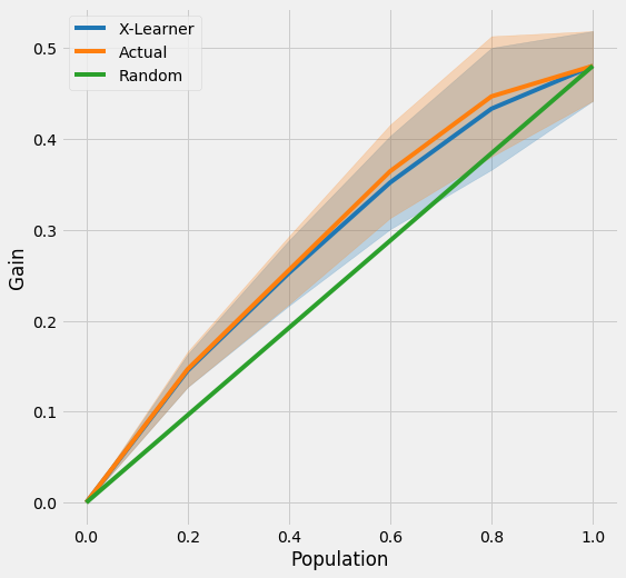
Uplift Curve with CI
[22]:
tmle_df = get_tmlegain(df, inference_col=inference_cols, outcome_col='y', treatment_col='w', p_col='p',
                       n_segment=5, cv=kf, ci=True)
[23]:
tmle_df
[23]:
| X-Learner | Actual | X-Learner LB | Actual LB | X-Learner UB | Actual UB | |
|---|---|---|---|---|---|---|
| 0.0 | 0.000000 | 0.000000 | 0.000000 | 0.000000 | 0.000000 | 0.000000 |
| 0.2 | 0.129817 | 0.137608 | 0.112298 | 0.118507 | 0.147336 | 0.156709 |
| 0.4 | 0.245069 | 0.260248 | 0.210048 | 0.223065 | 0.280090 | 0.297431 |
| 0.6 | 0.342145 | 0.360499 | 0.291017 | 0.309211 | 0.393274 | 0.411787 |
| 0.8 | 0.416171 | 0.424499 | 0.348987 | 0.358126 | 0.483356 | 0.490873 |
| 1.0 | 0.464096 | 0.464096 | 0.425783 | 0.425783 | 0.502409 | 0.502409 |
[24]:
plot_tmlegain(df, inference_col=inference_cols, outcome_col='y', treatment_col='w', p_col='p',
              n_segment=5, cv=kf, ci=True)
[25]:
plot(df, kind='gain', tmle=True, inference_col=inference_cols, outcome_col='y', treatment_col='w', p_col='p',
     n_segment=5, cv=kf, ci=True)

Qini Curve with TMLE as Ground Truth
Qini Curve without CI
[26]:
qini = get_tmleqini(df, inference_col=inference_cols, outcome_col='y', treatment_col='w', p_col='p',
                    n_segment=5, cv=kf, ci=False)
[27]:
qini
[27]:
| X-Learner | Actual | |
|---|---|---|
| 0.0 | 0.000000 | 0.000000 |
| 100000.0 | 44988.697939 | 56195.170032 |
| 200000.0 | 86989.528719 | 106484.749293 |
| 300000.0 | 116979.294111 | 132366.559586 |
| 400000.0 | 130594.141768 | 142357.640896 |
| 500000.0 | 120742.005413 | 120742.005413 |
[28]:
plot_tmleqini(df, inference_col=inference_cols, outcome_col='y', treatment_col='w', p_col='p',
              n_segment=5, cv=kf, ci=False)
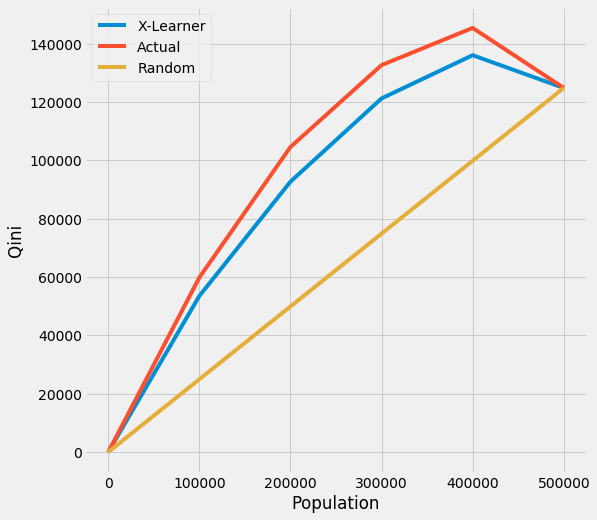
We also provide the api call directly with plot() by input kind='qini' and tmle=True
[29]:
plot(df, kind='qini', tmle=True, inference_col=inference_cols, outcome_col='y', treatment_col='w', p_col='p',
     n_segment=5, cv=kf, ci=False)

Qini Score
[30]:
qini_score(df, tmle=True, inference_col=inference_cols, outcome_col='y', treatment_col='w', p_col='p',
           n_segment=5, cv=kf, ci=False)
[30]:
X-Learner    23011.275285
Actual       32653.351497
dtype: float64
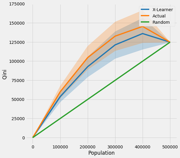
Qini Curve with CI
[31]:
qini = get_tmleqini(df, inference_col=inference_cols, outcome_col='y', treatment_col='w', p_col='p',
                    n_segment=5, cv=kf, ci=True)
[32]:
qini
[32]:
| X-Learner | Actual | X-Learner LB | Actual LB | X-Learner UB | Actual UB | |
|---|---|---|---|---|---|---|
| 0.0 | 0.000000 | 0.000000 | 0.000000 | 0.000000 | 0.000000 | 0.000000 |
| 100000.0 | 44988.697939 | 56195.170032 | 38917.392834 | 48394.895995 | 51060.003044 | 63995.444069 |
| 200000.0 | 86989.528719 | 106484.749293 | 74540.043943 | 91269.597859 | 99439.013495 | 121699.900726 |
| 300000.0 | 116979.294111 | 132366.559586 | 99553.599324 | 113510.079995 | 134404.988898 | 151223.039177 |
| 400000.0 | 130594.141768 | 142357.640896 | 110215.540730 | 121146.165100 | 150972.742806 | 163569.116693 |
| 500000.0 | 120742.005413 | 120742.005413 | 120742.005413 | 120742.005413 | 120742.005413 | 120742.005413 |
[33]:
plot_tmleqini(df, inference_col=inference_cols, outcome_col='y', treatment_col='w', p_col='p',
              n_segment=5, cv=kf, ci=True)

[34]:
plot(df, kind='qini', tmle=True, inference_col=inference_cols, outcome_col='y', treatment_col='w', p_col='p',
     n_segment=5, cv=kf, ci=True)