Causal Trees/Forests Treatment Effects Estimation and Tree Visualization

[1]:

import pandas as pd
import numpy as np
import multiprocessing as mp
from collections import defaultdict

np.random.seed(42)

from sklearn.model_selection import train_test_split
from sklearn.linear_model import LinearRegression
from sklearn.tree import DecisionTreeRegressor

import causalml
from causalml.metrics import plot_gain, plot_qini, qini_score
from causalml.dataset import synthetic_data
from causalml.inference.tree import plot_dist_tree_leaves_values, get_tree_leaves_mask
from causalml.inference.meta import BaseSRegressor, BaseXRegressor, BaseTRegressor, BaseDRRegressor
from causalml.inference.tree import CausalRandomForestRegressor
from causalml.inference.tree import CausalTreeRegressor
from causalml.inference.tree.plot import plot_causal_tree

import matplotlib.pyplot as plt
import seaborn as sns

%config InlineBackend.figure_format = 'retina'

Using `tqdm.autonotebook.tqdm` in notebook mode. Use `tqdm.tqdm` instead to force console mode (e.g. in jupyter console)
Failed to import duecredit due to No module named 'duecredit'

[2]:

import importlib
print(importlib.metadata.version('causalml') )

0.14.0

[3]:

# Simulate randomized trial: mode=2
y, X, w, tau, b, e = synthetic_data(mode=2, n=15000, p=20, sigma=5.5)

df = pd.DataFrame(X)
feature_names = [f'feature_{i}' for i in range(X.shape[1])]
df.columns = feature_names
df['outcome'] = y
df['treatment'] = w
df['treatment_effect'] = tau

[4]:

df.head()

[4]:

	feature_0	feature_1	feature_2	feature_3	feature_4	feature_5	feature_6	feature_7	feature_8	feature_9	...	feature_13	feature_14	feature_15	feature_16	feature_17	feature_18	feature_19	outcome	treatment	treatment_effect
0	0.496714	-0.138264	0.358450	1.523030	-0.234153	-0.234137	1.579213	0.767435	-0.469474	0.542560	...	-1.913280	-1.724918	-0.562288	-1.012831	0.314247	-0.908024	-1.412304	7.124356	1	1.123117
1	1.465649	-0.225776	1.239872	-1.424748	-0.544383	0.110923	-1.150994	0.375698	-0.600639	-0.291694	...	-1.057711	0.822545	-1.220844	0.208864	-1.959670	-1.328186	0.196861	-11.263144	0	2.052266
2	0.738467	0.171368	0.909835	-0.301104	-1.478522	-0.719844	-0.460639	1.057122	0.343618	-1.763040	...	0.611676	1.031000	0.931280	-0.839218	-0.309212	0.331263	0.975545	0.269378	0	1.520964
3	-0.479174	-0.185659	0.000000	-1.196207	0.812526	1.356240	-0.072010	1.003533	0.361636	-0.645120	...	1.564644	-2.619745	0.821903	0.087047	-0.299007	0.091761	-1.987569	-0.976893	0	0.125446
4	-0.219672	0.357113	0.137441	-0.518270	-0.808494	-0.501757	0.915402	0.328751	-0.529760	0.513267	...	-0.327662	-0.392108	-1.463515	0.296120	0.261055	0.005113	-0.234587	-1.949163	1	0.667889

5 rows × 23 columns

[5]:

# Look at the conversion rate and sample size in each group
df.pivot_table(values='outcome',
               index='treatment',
               aggfunc=[np.mean, np.size],
               margins=True)

[5]:

	mean	size
	outcome	outcome
treatment
0	0.736125	7502
1	1.543688	7498
All	1.139799	15000

[6]:

sns.kdeplot(data=df, x='outcome', hue='treatment')
plt.show()

../_images/examples_causal_trees_with_synthetic_data_6_0.png

[7]:

# Split data to training and testing samples for model validation (next section)
df_train, df_test = train_test_split(df, test_size=0.2, random_state=11101)
n_test = df_test.shape[0]
n_train = df_train.shape[0]

[8]:

# Table to gather estimated ITEs by models
df_result = pd.DataFrame({
    'outcome': df_test['outcome'],
    'is_treated': df_test['treatment'],
    'treatment_effect': df_test['treatment_effect']
})

CausalTreeRegressor

Available criteria for causal trees:

standard_mse: scikit-learn MSE where node values store \(E_{node_i}(X|T=1)-E_{node_i}(X|T=0)\), treatment effects.

causal_mse: The criteria reward a partition for finding strong heterogeneity in treatment effects and penalize a partition that creates variance in leaf estimates. https://www.pnas.org/doi/10.1073/pnas.1510489113

[9]:

ctrees = {
    'ctree_mse': {
        'params':
        dict(criterion='standard_mse',
             control_name=0,
             min_impurity_decrease=0,
             min_samples_leaf=400,
             groups_penalty=0.,
             groups_cnt=True),
    },
    'ctree_cmse': {
        'params':
        dict(
            criterion='causal_mse',
            control_name=0,
            min_samples_leaf=400,
            groups_penalty=0.,
            groups_cnt=True,
        ),
    },
    'ctree_cmse_p=0.1': {
        'params':
        dict(
            criterion='causal_mse',
            control_name=0,
            min_samples_leaf=400,
            groups_penalty=0.1,
            groups_cnt=True,
        ),
    },
    'ctree_cmse_p=0.25': {
        'params':
        dict(
            criterion='causal_mse',
            control_name=0,
            min_samples_leaf=400,
            groups_penalty=0.25,
            groups_cnt=True,
        ),
    },
    'ctree_cmse_p=0.5': {
        'params':
        dict(
            criterion='causal_mse',
            control_name=0,
            min_samples_leaf=400,
            groups_penalty=0.5,
            groups_cnt=True,
        ),
    },
    'ctree_ttest': {
        'params':
        dict(criterion='t_test',
             control_name=0,
             min_samples_leaf=400,
             groups_penalty=0.,
             groups_cnt=True),
    },
}

[10]:

# Model treatment effect
for ctree_name, ctree_info in ctrees.items():
    print(f"Fitting: {ctree_name}")
    ctree = CausalTreeRegressor(**ctree_info['params'])
    ctree.fit(X=df_train[feature_names].values,
              treatment=df_train['treatment'].values,
              y=df_train['outcome'].values)

    ctrees[ctree_name].update({'model': ctree})
    df_result[ctree_name] = ctree.predict(df_test[feature_names].values)

Fitting: ctree_mse
Fitting: ctree_cmse
Fitting: ctree_cmse_p=0.1
Fitting: ctree_cmse_p=0.25
Fitting: ctree_cmse_p=0.5
Fitting: ctree_ttest

[11]:

df_result.head()

[11]:

	outcome	is_treated	treatment_effect	ctree_mse	ctree_cmse	ctree_cmse_p=0.1	ctree_cmse_p=0.25	ctree_cmse_p=0.5	ctree_ttest
625	3.519424	1	0.819201	0.110685	0.895132	-1.104810	1.166407	1.166407	0.895132
5717	-1.175555	0	1.131599	0.183293	3.286218	2.071375	0.794040	0.794040	2.096099
14801	4.361167	0	1.969727	0.834163	3.329034	3.497691	3.097263	3.097263	2.077012
13605	4.523891	0	0.884079	0.183293	-0.727168	-2.025098	-0.902955	-0.902955	-0.727168
4208	-6.077212	0	1.179124	0.183293	3.329034	3.497691	1.916049	1.916049	1.257711

[12]:

# See treatment effect estimation with CausalTreeRegressor vs true treatment effect

n_obs = 300

indxs = df_result.index.values
np.random.shuffle(indxs)
indxs = indxs[:n_obs]

plt.rcParams.update({'font.size': 10})
pairplot = sns.pairplot(df_result[['treatment_effect', *list(ctrees)]])
pairplot.fig.suptitle(f"CausalTreeRegressor. Test sample size: {n_obs}" , y=1.02)
plt.show()

../_images/examples_causal_trees_with_synthetic_data_14_0.png

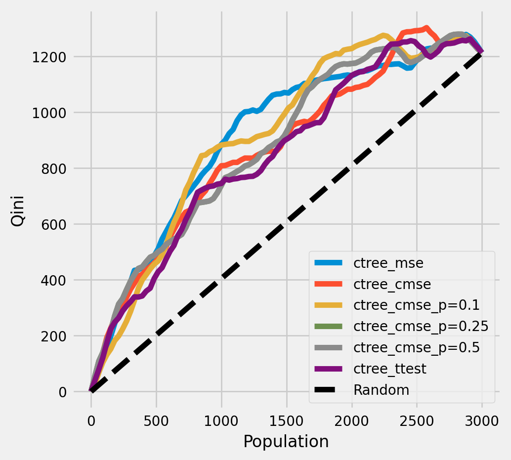
Plot the Qini chart

[13]:

plot_qini(df_result,
          outcome_col='outcome',
          treatment_col='is_treated',
          treatment_effect_col='treatment_effect',
          figsize=(5,5)
         )

../_images/examples_causal_trees_with_synthetic_data_16_0.png

[14]:

df_qini = qini_score(df_result,
           outcome_col='outcome',
           treatment_col='is_treated',
           treatment_effect_col='treatment_effect')
df_qini.sort_values(ascending=False)

[14]:

ctree_cmse_p=0.1     0.273112
ctree_mse            0.260141
ctree_ttest          0.247668
ctree_cmse           0.242333
ctree_cmse_p=0.25    0.231232
ctree_cmse_p=0.5     0.231232
Random               0.000000
dtype: float64

The cumulative gain of the true treatment effect in each population

[15]:

plot_gain(df_result,
          outcome_col='outcome',
          treatment_col='is_treated',
          treatment_effect_col='treatment_effect',
          n = n_test,
          figsize=(5,5)
         )

../_images/examples_causal_trees_with_synthetic_data_19_0.png

The cumulative difference between the mean outcomes of the treatment and control groups in each population

[16]:

plot_gain(df_result,
          outcome_col='outcome',
          treatment_col='is_treated',
          n = n_test,
          figsize=(5,5)
         )

../_images/examples_causal_trees_with_synthetic_data_21_0.png

Plot trees with sklearn function and save as vector graphics

[17]:

for ctree_name, ctree_info in ctrees.items():
    plt.figure(figsize=(20,20))
    plot_causal_tree(ctree_info['model'],
                     feature_names = feature_names,
                     filled=True,
                     impurity=True,
                     proportion=False,
              )
    plt.title(ctree_name)
    plt.savefig(f'{ctree_name}.svg')

../_images/examples_causal_trees_with_synthetic_data_23_0.png

../_images/examples_causal_trees_with_synthetic_data_23_1.png

../_images/examples_causal_trees_with_synthetic_data_23_2.png

../_images/examples_causal_trees_with_synthetic_data_23_3.png

../_images/examples_causal_trees_with_synthetic_data_23_4.png

../_images/examples_causal_trees_with_synthetic_data_23_5.png

How values in leaves of the fitted trees differ from each other:

[18]:

for ctree_name, ctree_info in ctrees.items():
    plot_dist_tree_leaves_values(ctree_info['model'],
                                 figsize=(3,3),
                                 title=f'Tree({ctree_name}) leaves values distribution')

../_images/examples_causal_trees_with_synthetic_data_25_0.png

../_images/examples_causal_trees_with_synthetic_data_25_1.png

../_images/examples_causal_trees_with_synthetic_data_25_2.png

../_images/examples_causal_trees_with_synthetic_data_25_3.png

../_images/examples_causal_trees_with_synthetic_data_25_4.png

../_images/examples_causal_trees_with_synthetic_data_25_5.png

CausalRandomForestRegressor

[19]:

cforests = {
    'cforest_mse': {
        'params':
        dict(criterion='standard_mse',
             control_name=0,
             min_impurity_decrease=0,
             min_samples_leaf=400,
             groups_penalty=0.,
             groups_cnt=True),
    },
    'cforest_cmse': {
        'params':
        dict(
            criterion='causal_mse',
            control_name=0,
            min_samples_leaf=400,
            groups_penalty=0.,
            groups_cnt=True
        ),
    },
    'cforest_cmse_p=0.5': {
        'params':
        dict(
            criterion='causal_mse',
            control_name=0,
            min_samples_leaf=400,
            groups_penalty=0.5,
            groups_cnt=True,
        ),
    },
    'cforest_cmse_p=0.5_md=3': {
        'params':
        dict(
            criterion='causal_mse',
            control_name=0,
            max_depth=3,
            min_samples_leaf=400,
            groups_penalty=0.5,
            groups_cnt=True,
        ),
    },
    'cforest_ttest': {
        'params':
        dict(criterion='t_test',
             control_name=0,
             min_samples_leaf=400,
             groups_penalty=0.,
             groups_cnt=True),
    },
}

[20]:

# Model treatment effect
for cforest_name, cforest_info in cforests.items():
    print(f"Fitting: {cforest_name}")
    cforest = CausalRandomForestRegressor(**cforest_info['params'])
    cforest.fit(X=df_train[feature_names].values,
              treatment=df_train['treatment'].values,
              y=df_train['outcome'].values)

    cforests[cforest_name].update({'model': cforest})
    df_result[cforest_name] = cforest.predict(df_test[feature_names].values)

Fitting: cforest_mse
Fitting: cforest_cmse
Fitting: cforest_cmse_p=0.5
Fitting: cforest_cmse_p=0.5_md=3
Fitting: cforest_ttest

[21]:

# See treatment effect estimation with CausalRandomForestRegressor vs true treatment effect

n_obs = 200

indxs = df_result.index.values
np.random.shuffle(indxs)
indxs = indxs[:n_obs]

plt.rcParams.update({'font.size': 10})
pairplot = sns.pairplot(df_result[['treatment_effect', *list(cforests)]])
pairplot.fig.suptitle(f"CausalRandomForestRegressor. Test sample size: {n_obs}" , y=1.02)
plt.show()

../_images/examples_causal_trees_with_synthetic_data_29_0.png

[22]:

df_qini = qini_score(df_result,
           outcome_col='outcome',
           treatment_col='is_treated',
           treatment_effect_col='treatment_effect')

df_qini.sort_values(ascending=False)

[22]:

cforest_cmse_p=0.5_md=3    0.379598
cforest_cmse_p=0.5         0.344870
cforest_ttest              0.329592
cforest_mse                0.326770
cforest_cmse               0.323620
ctree_cmse_p=0.1           0.273112
ctree_mse                  0.260141
ctree_ttest                0.247668
ctree_cmse                 0.242333
ctree_cmse_p=0.25          0.231232
ctree_cmse_p=0.5           0.231232
Random                     0.000000
dtype: float64

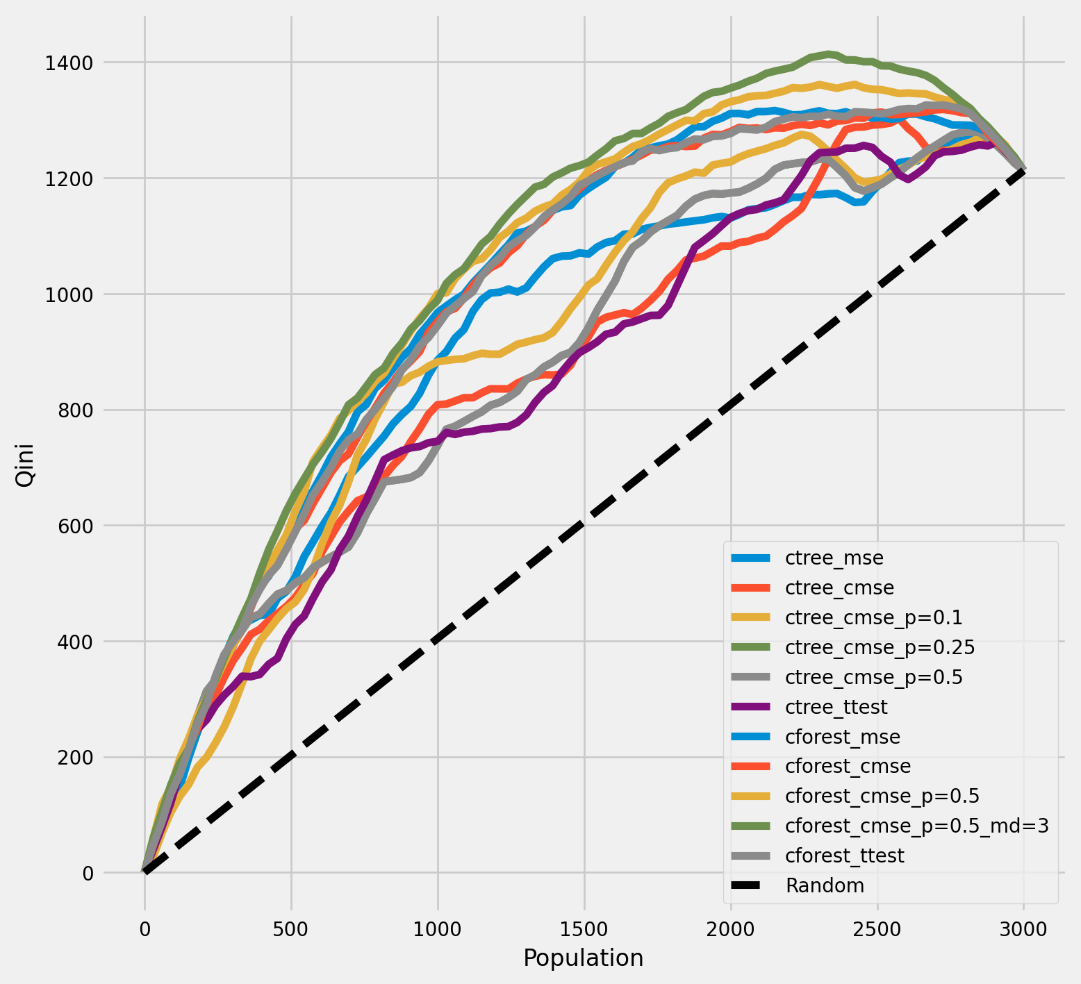
Qini chart

[23]:

plot_qini(df_result,
          outcome_col='outcome',
          treatment_col='is_treated',
          treatment_effect_col='treatment_effect',
          figsize=(8,8)
         )

../_images/examples_causal_trees_with_synthetic_data_32_0.png

[24]:

df_qini = qini_score(df_result,
           outcome_col='outcome',
           treatment_col='is_treated',
           treatment_effect_col='treatment_effect')

df_qini.sort_values(ascending=False)

[24]:

cforest_cmse_p=0.5_md=3    0.379598
cforest_cmse_p=0.5         0.344870
cforest_ttest              0.329592
cforest_mse                0.326770
cforest_cmse               0.323620
ctree_cmse_p=0.1           0.273112
ctree_mse                  0.260141
ctree_ttest                0.247668
ctree_cmse                 0.242333
ctree_cmse_p=0.25          0.231232
ctree_cmse_p=0.5           0.231232
Random                     0.000000
dtype: float64

The cumulative gain of the true treatment effect in each population

[25]:

plot_gain(df_result,
          outcome_col='outcome',
          treatment_col='is_treated',
          treatment_effect_col='treatment_effect',
          n = n_test
         )

../_images/examples_causal_trees_with_synthetic_data_35_0.png

The cumulative difference between the mean outcomes of the treatment and control groups in each population

[26]:

plot_gain(df_result,
          outcome_col='outcome',
          treatment_col='is_treated',
          n = n_test
         )

../_images/examples_causal_trees_with_synthetic_data_37_0.png

Meta-Learner Algorithms

[27]:

X_train = df_train[feature_names].values
X_test = df_test[feature_names].values

# learner - DecisionTreeRegressor
# treatment learner - LinearRegression()

learner_x = BaseXRegressor(learner=DecisionTreeRegressor(),
                           treatment_effect_learner=LinearRegression())
learner_s = BaseSRegressor(learner=DecisionTreeRegressor())
learner_t = BaseTRegressor(learner=DecisionTreeRegressor(),
                           treatment_learner=LinearRegression())
learner_dr = BaseDRRegressor(learner=DecisionTreeRegressor(),
                             treatment_effect_learner=LinearRegression())

learner_x.fit(X=X_train, treatment=df_train['treatment'].values, y=df_train['outcome'].values)
learner_s.fit(X=X_train, treatment=df_train['treatment'].values, y=df_train['outcome'].values)
learner_t.fit(X=X_train, treatment=df_train['treatment'].values, y=df_train['outcome'].values)
learner_dr.fit(X=X_train, treatment=df_train['treatment'].values, y=df_train['outcome'].values)

df_result['learner_x_ite'] = learner_x.predict(X_test)
df_result['learner_s_ite'] = learner_s.predict(X_test)
df_result['learner_t_ite'] = learner_t.predict(X_test)
df_result['learner_dr_ite'] = learner_dr.predict(X_test)

[28]:

cate_dr = learner_dr.predict(X)
cate_x = learner_x.predict(X)
cate_s = learner_s.predict(X)
cate_t = learner_t.predict(X)

cate_ctrees = [info['model'].predict(X) for _, info in ctrees.items()]
cate_cforests = [info['model'].predict(X) for _, info in cforests.items()]

model_cate = [
    *cate_ctrees,
    *cate_cforests,
    cate_x, cate_s, cate_t, cate_dr
]

model_names = [
    *list(ctrees), *list(cforests),
    'X Learner', 'S Learner', 'T Learner', 'DR Learner']

[29]:

plot_gain(df_result,
          outcome_col='outcome',
          treatment_col='is_treated',
          n = n_test
         )

../_images/examples_causal_trees_with_synthetic_data_41_0.png

[30]:

rows = 2
cols = 7
row_idxs = np.arange(rows)
col_idxs = np.arange(cols)

ax_idxs = np.dstack(np.meshgrid(col_idxs, row_idxs)).reshape(-1, 2)

[31]:

fig, ax = plt.subplots(rows, cols, figsize=(20, 10))
plt.rcParams.update({'font.size': 10})

for ax_idx, cate, model_name in zip(ax_idxs, model_cate, model_names):
    col_id, row_id = ax_idx
    cur_ax = ax[row_id, col_id]
    cur_ax.scatter(tau, cate, alpha=0.3)
    cur_ax.plot(tau, tau, color='C2', linewidth=2)
    cur_ax.set_xlabel('True ITE')
    cur_ax.set_ylabel('Estimated ITE')
    cur_ax.set_title(model_name)
    cur_ax.set_xlim((-4, 6))

../_images/examples_causal_trees_with_synthetic_data_43_0.png

The cumulative difference between the mean outcomes of the treatment and control groups in each population

[32]:

plot_gain(df_result,
          outcome_col='outcome',
          treatment_col='is_treated',
          n = n_test,
          figsize=(9, 9),
         )

../_images/examples_causal_trees_with_synthetic_data_45_0.png

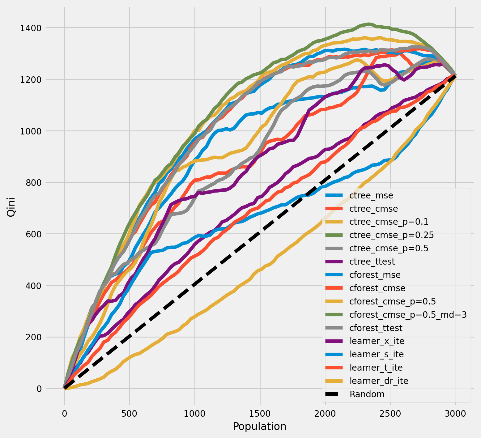
Qini chart

[33]:

plot_qini(df_result,
          outcome_col='outcome',
          treatment_col='is_treated',
          treatment_effect_col='treatment_effect',
         )

../_images/examples_causal_trees_with_synthetic_data_47_0.png

[34]:

df_qini = qini_score(df_result,
           outcome_col='outcome',
           treatment_col='is_treated',
           treatment_effect_col='treatment_effect')
df_qini.sort_values(ascending=False)

[34]:

cforest_cmse_p=0.5_md=3    0.379598
learner_dr_ite             0.350053
cforest_cmse_p=0.5         0.344870
cforest_ttest              0.329592
cforest_mse                0.326770
cforest_cmse               0.323620
ctree_cmse_p=0.1           0.273112
ctree_mse                  0.260141
ctree_ttest                0.247668
ctree_cmse                 0.242333
ctree_cmse_p=0.25          0.231232
ctree_cmse_p=0.5           0.231232
learner_x_ite              0.096785
learner_t_ite              0.082948
learner_s_ite              0.055251
Random                     0.000000
dtype: float64

Return outcomes along with estimated treatment effects

[35]:

ctree_outcomes = ctrees["ctree_mse"]["model"].predict(X_test, with_outcomes=True)
df_ctree_outcomes = pd.DataFrame(ctree_outcomes, columns=["Y0", "Y1", "ITE"])
df_ctree_outcomes.head()

[35]:

	Y0	Y1	ITE
0	0.434715	0.545400	0.110685
1	1.825205	2.008497	0.183293
2	0.453153	1.287316	0.834163
3	1.825205	2.008497	0.183293
4	1.825205	2.008497	0.183293

[36]:

cforest_outcomes = cforests["cforest_mse"]["model"].predict(X_test, with_outcomes=True)
df_cforest_outcomes = pd.DataFrame(cforest_outcomes, columns=["Y0", "Y1", "ITE"])
df_cforest_outcomes.head()

[36]:

	Y0	Y1	ITE
0	0.390998	0.575902	0.184904
1	1.445800	1.852422	0.406622
2	0.385520	0.982415	0.596895
3	1.279227	1.731512	0.452285
4	1.279100	1.730838	0.451738

Bootstrap confidence intervals for individual treatment effects

[37]:

alpha=0.05
tree = CausalTreeRegressor(criterion='causal_mse', control_name=0, min_samples_leaf=200, alpha=alpha)

[38]:

# For time measurements
for n_jobs in (4, mp.cpu_count() - 1):
    for n_bootstraps in (10, 50, 100):
        print(f"n_jobs: {n_jobs} n_bootstraps: {n_bootstraps}" )
        tree.bootstrap_pool(
            X=X,
            treatment=w,
            y=y,
            n_bootstraps=n_bootstraps,
            bootstrap_size=10000,
            n_jobs=n_jobs,
            verbose=False
        )

n_jobs: 4 n_bootstraps: 10

100%|██████████████████████████████████████████████████████████████████████████████████████████████████████████████████████████████████████████████████████████████████████████████████████████| 10/10 [00:00<00:00, 20.81it/s]

Function: bootstrap_pool Kwargs:{'n_bootstraps': 10, 'bootstrap_size': 10000, 'n_jobs': 4, 'verbose': False} Elapsed time: 0.9135
n_jobs: 4 n_bootstraps: 50


100%|██████████████████████████████████████████████████████████████████████████████████████████████████████████████████████████████████████████████████████████████████████████████████████████| 50/50 [00:02<00:00, 21.29it/s]

Function: bootstrap_pool Kwargs:{'n_bootstraps': 50, 'bootstrap_size': 10000, 'n_jobs': 4, 'verbose': False} Elapsed time: 2.4252
n_jobs: 4 n_bootstraps: 100


100%|████████████████████████████████████████████████████████████████████████████████████████████████████████████████████████████████████████████████████████████████████████████████████████| 100/100 [00:04<00:00, 21.70it/s]

Function: bootstrap_pool Kwargs:{'n_bootstraps': 100, 'bootstrap_size': 10000, 'n_jobs': 4, 'verbose': False} Elapsed time: 4.6932
n_jobs: 11 n_bootstraps: 10


100%|██████████████████████████████████████████████████████████████████████████████████████████████████████████████████████████████████████████████████████████████████████████████████████████| 10/10 [00:00<00:00, 32.93it/s]

Function: bootstrap_pool Kwargs:{'n_bootstraps': 10, 'bootstrap_size': 10000, 'n_jobs': 11, 'verbose': False} Elapsed time: 0.6439
n_jobs: 11 n_bootstraps: 50


100%|██████████████████████████████████████████████████████████████████████████████████████████████████████████████████████████████████████████████████████████████████████████████████████████| 50/50 [00:01<00:00, 30.42it/s]

Function: bootstrap_pool Kwargs:{'n_bootstraps': 50, 'bootstrap_size': 10000, 'n_jobs': 11, 'verbose': False} Elapsed time: 1.8508
n_jobs: 11 n_bootstraps: 100


100%|████████████████████████████████████████████████████████████████████████████████████████████████████████████████████████████████████████████████████████████████████████████████████████| 100/100 [00:02<00:00, 33.67it/s]

Function: bootstrap_pool Kwargs:{'n_bootstraps': 100, 'bootstrap_size': 10000, 'n_jobs': 11, 'verbose': False} Elapsed time: 3.1553

[39]:

te, te_lower, te_upper = tree.fit_predict(
        X=df_train[feature_names].values,
        treatment=df_train["treatment"].values,
        y=df_train["outcome"].values,
        return_ci=True,
        n_bootstraps=500,
        bootstrap_size=5000,
        n_jobs=mp.cpu_count() - 1,
        verbose=False)

100%|████████████████████████████████████████████████████████████████████████████████████████████████████████████████████████████████████████████████████████████████████████████████████████| 500/500 [00:06<00:00, 81.19it/s]

Function: bootstrap_pool Kwargs:{'n_bootstraps': 500, 'bootstrap_size': 5000, 'n_jobs': 11, 'verbose': False} Elapsed time: 6.4025

[40]:

plt.hist(te_lower, color='red', alpha=0.3, label='lower_bound')
plt.axvline(x = 0, color = 'black', linestyle='--', lw=1, label='')
plt.legend()
plt.show()

../_images/examples_causal_trees_with_synthetic_data_57_0.png

[41]:

# Significant estimates for negative and positive individual effects
# Default alpha = 0.05

bootstrap_neg = te[(te_lower < 0) & (te_upper < 0)]
bootstrap_pos = te[(te_lower > 0) & (te_upper > 0)]
print(bootstrap_neg.shape, bootstrap_pos.shape)

(0,) (7,)

[42]:

plt.hist(bootstrap_neg)
plt.title(f'Bootstrap-based subsample of significant negative ITE. alpha={alpha}')
plt.show()

plt.hist(bootstrap_pos)
plt.title(f'Bootstrap-based subsample of significant positive ITE alpha={alpha}')
plt.show()

../_images/examples_causal_trees_with_synthetic_data_59_0.png

../_images/examples_causal_trees_with_synthetic_data_59_1.png

Average treatment effect

[43]:

tree = CausalTreeRegressor(criterion='causal_mse', control_name=0, min_samples_leaf=200, alpha=alpha)
te, te_lb, te_ub = tree.estimate_ate(X=X, treatment=w, y=y)
print('ATE:', te, 'Bounds:', (te_lb, te_ub ), 'alpha:', alpha)

ATE: 0.80899590297471 Bounds: (0.808752005241054, 0.8092398007083661) alpha: 0.05

CausalRandomForestRegressor ITE std

[44]:

crforest = CausalRandomForestRegressor(criterion="causal_mse",  min_samples_leaf=200,
                                       control_name=0, n_estimators=50, n_jobs=mp.cpu_count()-1)
crforest.fit(X=df_train[feature_names].values,
             treatment=df_train['treatment'].values,
             y=df_train['outcome'].values
             )

[44]:

CausalRandomForestRegressor(min_samples_leaf=200, n_estimators=50, n_jobs=11)

[45]:

crforest_te_pred = crforest.predict(df_test[feature_names])
crforest_test_var = crforest.calculate_error(X_train=df_train[feature_names].values,
                                        X_test=df_test[feature_names].values)
crforest_test_std = np.sqrt(crforest_test_var)

[46]:

plt.hist(crforest_test_std)
plt.title("CausalRandomForestRegressor unbiased sampling std")
plt.show()

../_images/examples_causal_trees_with_synthetic_data_65_0.png

[ ]:

[ ]:

Read the Docs v: latest

Versions: latest; stable; huigang-doc_update

Downloads: pdf; html; epub

On Read the Docs: Project Home; Builds