Uplift Trees Example with Synthetic Data

In this notebook, we use synthetic data to demonstrate the use of the tree-based algorithms.

import numpy as np
import pandas as pd

from causalml.dataset import make_uplift_classification
from causalml.inference.tree import UpliftRandomForestClassifier
from causalml.metrics import plot_gain

from sklearn.model_selection import train_test_split

import importlib
print(importlib.metadata.version('causalml') )

0.14.0

Generate synthetic dataset

The CausalML package contains various functions to generate synthetic datasets for uplift modeling. Here we generate a classification dataset using the make_uplift_classification() function.

df, x_names = make_uplift_classification()

df.head()

	treatment_group_key	x1_informative	x2_informative	x3_informative	x4_informative	x5_informative	x6_irrelevant	x7_irrelevant	x8_irrelevant	x9_irrelevant	...	x12_uplift_increase	x13_increase_mix	x14_uplift_increase	x15_uplift_increase	x16_increase_mix	x17_uplift_increase	x18_uplift_increase	x19_increase_mix	conversion	treatment_effect
0	control	-0.542888	1.976361	-0.531359	-2.354211	-0.380629	-2.614321	-0.128893	0.448689	-2.275192	...	-1.315304	0.742654	1.891699	-2.428395	1.541875	-0.817705	-0.610194	-0.591581	0	0
1	treatment3	0.258654	0.552412	1.434239	-1.422311	0.089131	0.790293	1.159513	1.578868	0.166540	...	-1.391878	-0.623243	2.443972	-2.889253	2.018585	-1.109296	-0.380362	-1.667606	0	0
2	treatment1	1.697012	-2.762600	-0.662874	-1.682340	1.217443	0.837982	1.042981	0.177398	-0.112409	...	-1.132497	1.050179	1.573054	-1.788427	1.341609	-0.749227	-2.091521	-0.471386	0	0
3	treatment2	-1.441644	1.823648	0.789423	-0.295398	0.718509	-0.492993	0.947824	-1.307887	0.123340	...	-2.084619	0.058481	1.369439	0.422538	1.087176	-0.966666	-1.785592	-1.268379	1	1
4	control	-0.625074	3.002388	-0.096288	1.938235	3.392424	-0.465860	-0.919897	-1.072592	-1.331181	...	-1.403984	0.760430	1.917635	-2.347675	1.560946	-0.833067	-1.407884	-0.781343	0	0

5 rows × 22 columns

# Look at the conversion rate and sample size in each group
df.pivot_table(values='conversion',
               index='treatment_group_key',
               aggfunc=[np.mean, np.size],
               margins=True)

	mean	size
	conversion	conversion
treatment_group_key
control	0.511	1000
treatment1	0.514	1000
treatment2	0.559	1000
treatment3	0.600	1000
All	0.546	4000

Run the uplift random forest classifier

In this section, we first fit the uplift random forest classifier using training data. We then use the fitted model to make a prediction using testing data. The prediction returns an ndarray in which each column contains the predicted uplift if the unit was in the corresponding treatment group.

# Split data to training and testing samples for model validation (next section)
df_train, df_test = train_test_split(df, test_size=0.2, random_state=111)

from causalml.inference.tree import UpliftTreeClassifier

clf = UpliftTreeClassifier(control_name='control')
clf.fit(df_train[x_names].values,
         treatment=df_train['treatment_group_key'].values,
         y=df_train['conversion'].values)
p = clf.predict(df_test[x_names].values)

df_res = pd.DataFrame(p, columns=clf.classes_)
df_res.head()

	control	treatment1	treatment2	treatment3
0	0.506394	0.511811	0.573935	0.503778
1	0.506394	0.511811	0.573935	0.503778
2	0.580838	0.458824	0.508982	0.452381
3	0.482558	0.572327	0.556757	0.961538
4	0.482558	0.572327	0.556757	0.961538

uplift_model = UpliftRandomForestClassifier(control_name='control')

uplift_model.fit(df_train[x_names].values,
                 treatment=df_train['treatment_group_key'].values,
                 y=df_train['conversion'].values)

df_res = uplift_model.predict(df_test[x_names].values, full_output=True)
print(df_res.shape)
df_res.head()

(800, 9)

	control	treatment1	treatment2	treatment3	recommended_treatment	delta_treatment1	delta_treatment2	delta_treatment3	max_delta
0	0.415263	0.401823	0.465554	0.391658	2	-0.013440	0.050291	-0.023605	0.050291
1	0.412962	0.389346	0.476169	0.363343	2	-0.023616	0.063206	-0.049619	0.063206
2	0.533442	0.548670	0.589756	0.588654	2	0.015228	0.056313	0.055212	0.056313
3	0.344854	0.314433	0.370315	0.760676	3	-0.030420	0.025461	0.415822	0.415822
4	0.649657	0.602642	0.641364	0.851301	3	-0.047015	-0.008293	0.201644	0.201644

y_pred = uplift_model.predict(df_test[x_names].values)

y_pred.shape

(800, 3)

# Put the predictions to a DataFrame for a neater presentation
# The output of `predict()` is a numpy array with the shape of [n_sample, n_treatment] excluding the
# predictions for the control group.
result = pd.DataFrame(y_pred,
                      columns=uplift_model.classes_[1:])
result.head()

	treatment1	treatment2	treatment3
0	-0.013440	0.050291	-0.023605
1	-0.023616	0.063206	-0.049619
2	0.015228	0.056313	0.055212
3	-0.030420	0.025461	0.415822
4	-0.047015	-0.008293	0.201644

Create the uplift curve

The performance of the model can be evaluated with the help of the uplift curve.

Create a synthetic population

The uplift curve is calculated on a synthetic population that consists of those that were in the control group and those who happened to be in the treatment group recommended by the model. We use the synthetic population to calculate the actual treatment effect within predicted treatment effect quantiles. Because the data is randomized, we have a roughly equal number of treatment and control observations in the predicted quantiles and there is no self selection to treatment groups.

# If all deltas are negative, assing to control; otherwise assign to the treatment
# with the highest delta
best_treatment = np.where((result < 0).all(axis=1),
                           'control',
                           result.idxmax(axis=1))

# Create indicator variables for whether a unit happened to have the
# recommended treatment or was in the control group
actual_is_best = np.where(df_test['treatment_group_key'] == best_treatment, 1, 0)
actual_is_control = np.where(df_test['treatment_group_key'] == 'control', 1, 0)

synthetic = (actual_is_best == 1) | (actual_is_control == 1)
synth = result[synthetic]

Calculate the observed treatment effect per predicted treatment effect quantile

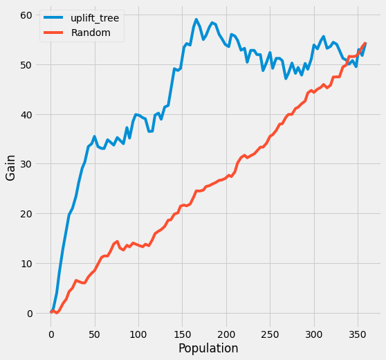
We use the observed treatment effect to calculate the uplift curve, which answers the question: how much of the total cumulative uplift could we have captured by targeting a subset of the population sorted according to the predicted uplift, from highest to lowest?

CausalML has the plot_gain() function which calculates the uplift curve given a DataFrame containing the treatment assignment, observed outcome and the predicted treatment effect.

auuc_metrics = (synth.assign(is_treated = 1 - actual_is_control[synthetic],
                             conversion = df_test.loc[synthetic, 'conversion'].values,
                             uplift_tree = synth.max(axis=1))
                     .drop(columns=list(uplift_model.classes_[1:])))

plot_gain(auuc_metrics, outcome_col='conversion', treatment_col='is_treated')