Sensitivity Analysis Examples

Methods

We provided five methods for sensitivity analysis including (Placebo Treatment, Random Cause, Subset Data, Random Replace and Selection Bias). This notebook will walkthrough how to use the combined function sensitivity_analysis() to compare different method and also how to use each individual method separately:

Placebo Treatment: Replacing treatment with a random variable
Irrelevant Additional Confounder: Adding a random common cause variable
Subset validation: Removing a random subset of the data
Selection Bias method with One Sided confounding function and Alignment confounding function
Random Replace: Random replace a covariate with an irrelevant variable

[2]:

%matplotlib inline
%load_ext autoreload
%autoreload 2

[3]:

import pandas as pd
import matplotlib.pyplot as plt
from sklearn.linear_model import LinearRegression
import warnings
import matplotlib
from causalml.inference.meta import BaseXLearner
from causalml.dataset import synthetic_data

from causalml.metrics.sensitivity import Sensitivity
from causalml.metrics.sensitivity import SensitivityRandomReplace, SensitivitySelectionBias

plt.style.use('fivethirtyeight')
matplotlib.rcParams['figure.figsize'] = [8, 8]
warnings.filterwarnings('ignore')

# logging.basicConfig(level=logging.INFO)

pd.options.display.float_format = '{:.4f}'.format

/Users/jing.pan/anaconda3/envs/causalml_3_6/lib/python3.6/site-packages/sklearn/utils/deprecation.py:144: FutureWarning: The sklearn.utils.testing module is  deprecated in version 0.22 and will be removed in version 0.24. The corresponding classes / functions should instead be imported from sklearn.utils. Anything that cannot be imported from sklearn.utils is now part of the private API.
  warnings.warn(message, FutureWarning)

Generate Synthetic data

[4]:

# Generate synthetic data using mode 1
num_features = 6
y, X, treatment, tau, b, e = synthetic_data(mode=1, n=100000, p=num_features, sigma=1.0)

[5]:

tau.mean()

[5]:

0.5001096146567363

Define Features

[6]:

# Generate features names
INFERENCE_FEATURES = ['feature_' + str(i) for i in range(num_features)]
TREATMENT_COL = 'target'
OUTCOME_COL = 'outcome'
SCORE_COL = 'pihat'

[7]:

df = pd.DataFrame(X, columns=INFERENCE_FEATURES)
df[TREATMENT_COL] = treatment
df[OUTCOME_COL] = y
df[SCORE_COL] = e

[8]:

df.head()

[8]:

	feature_0	feature_1	feature_2	feature_3	feature_4	feature_5	target	outcome	pihat
0	0.9536	0.2911	0.0432	0.8720	0.5190	0.0822	1	2.0220	0.7657
1	0.2390	0.3096	0.5115	0.2048	0.8914	0.5015	0	-0.0732	0.2304
2	0.1091	0.0765	0.7428	0.6951	0.4580	0.7800	0	-1.4947	0.1000
3	0.2055	0.3967	0.6278	0.2086	0.3865	0.8860	0	0.6458	0.2533
4	0.4501	0.0578	0.3972	0.4100	0.5760	0.4764	0	-0.0018	0.1000

With all Covariates

Sensitivity Analysis Summary Report (with One-sided confounding function and default alpha)

[9]:

# Calling the Base XLearner class and return the sensitivity analysis summary report
learner_x = BaseXLearner(LinearRegression())
sens_x = Sensitivity(df=df, inference_features=INFERENCE_FEATURES, p_col='pihat',
                     treatment_col=TREATMENT_COL, outcome_col=OUTCOME_COL, learner=learner_x)
# Here for Selection Bias method will use default one-sided confounding function and alpha (quantile range of outcome values) input
sens_sumary_x = sens_x.sensitivity_analysis(methods=['Placebo Treatment',
                                                     'Random Cause',
                                                     'Subset Data',
                                                     'Random Replace',
                                                     'Selection Bias'], sample_size=0.5)

[10]:

# From the following results, refutation methods show our model is pretty robust;
# When alpah > 0, the treated group always has higher mean potential outcomes than the control; when  < 0, the control group is better off.
sens_sumary_x

[10]:

	Method	ATE	New ATE	New ATE LB	New ATE UB
0	Placebo Treatment	0.6801	-0.0025	-0.0158	0.0107
0	Random Cause	0.6801	0.6801	0.6673	0.6929
0	Subset Data(sample size @0.5)	0.6801	0.6874	0.6693	0.7055
0	Random Replace	0.6801	0.6799	0.6670	0.6929
0	Selection Bias (alpha@-0.80111, with r-sqaure:...	0.6801	1.3473	1.3347	1.3599
0	Selection Bias (alpha@-0.64088, with r-sqaure:...	0.6801	1.2139	1.2013	1.2265
0	Selection Bias (alpha@-0.48066, with r-sqaure:...	0.6801	1.0804	1.0678	1.0931
0	Selection Bias (alpha@-0.32044, with r-sqaure:...	0.6801	0.9470	0.9343	0.9597
0	Selection Bias (alpha@-0.16022, with r-sqaure:...	0.6801	0.8135	0.8008	0.8263
0	Selection Bias (alpha@0.0, with r-sqaure:0.0	0.6801	0.6801	0.6673	0.6929
0	Selection Bias (alpha@0.16022, with r-sqaure:0...	0.6801	0.5467	0.5338	0.5595
0	Selection Bias (alpha@0.32044, with r-sqaure:0...	0.6801	0.4132	0.4003	0.4261
0	Selection Bias (alpha@0.48066, with r-sqaure:0...	0.6801	0.2798	0.2668	0.2928
0	Selection Bias (alpha@0.64088, with r-sqaure:0...	0.6801	0.1463	0.1332	0.1594
0	Selection Bias (alpha@0.80111, with r-sqaure:0...	0.6801	0.0129	-0.0003	0.0261

Random Replace

[11]:

# Replace feature_0 with an irrelevent variable
sens_x_replace = SensitivityRandomReplace(df=df, inference_features=INFERENCE_FEATURES, p_col='pihat',
                                          treatment_col=TREATMENT_COL, outcome_col=OUTCOME_COL, learner=learner_x,
                                          sample_size=0.9, replaced_feature='feature_0')
s_check_replace = sens_x_replace.summary(method='Random Replace')
s_check_replace

[11]:

	Method	ATE	New ATE	New ATE LB	New ATE UB
0	Random Replace	0.6801	0.8072	0.7943	0.8200

Selection Bias: Alignment confounding Function

[12]:

sens_x_bias_alignment = SensitivitySelectionBias(df, INFERENCE_FEATURES, p_col='pihat', treatment_col=TREATMENT_COL,
                                                 outcome_col=OUTCOME_COL, learner=learner_x, confound='alignment',
                                                 alpha_range=None)

[13]:

lls_x_bias_alignment, partial_rsqs_x_bias_alignment = sens_x_bias_alignment.causalsens()

[14]:

lls_x_bias_alignment

[14]:

	alpha	rsqs	New ATE	New ATE LB	New ATE UB
0	-0.8011	0.1088	0.6685	0.6556	0.6813
0	-0.6409	0.0728	0.6708	0.6580	0.6836
0	-0.4807	0.0425	0.6731	0.6604	0.6859
0	-0.3204	0.0194	0.6754	0.6627	0.6882
0	-0.1602	0.0050	0.6778	0.6650	0.6905
0	0.0000	0.0000	0.6801	0.6673	0.6929
0	0.1602	0.0050	0.6824	0.6696	0.6953
0	0.3204	0.0200	0.6848	0.6718	0.6977
0	0.4807	0.0443	0.6871	0.6741	0.7001
0	0.6409	0.0769	0.6894	0.6763	0.7026
0	0.8011	0.1164	0.6918	0.6785	0.7050

[15]:

partial_rsqs_x_bias_alignment

[15]:

	feature	partial_rsqs
0	feature_0	-0.0631
1	feature_1	-0.0619
2	feature_2	-0.0001
3	feature_3	-0.0033
4	feature_4	-0.0001
5	feature_5	0.0000

[16]:

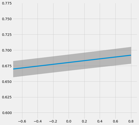
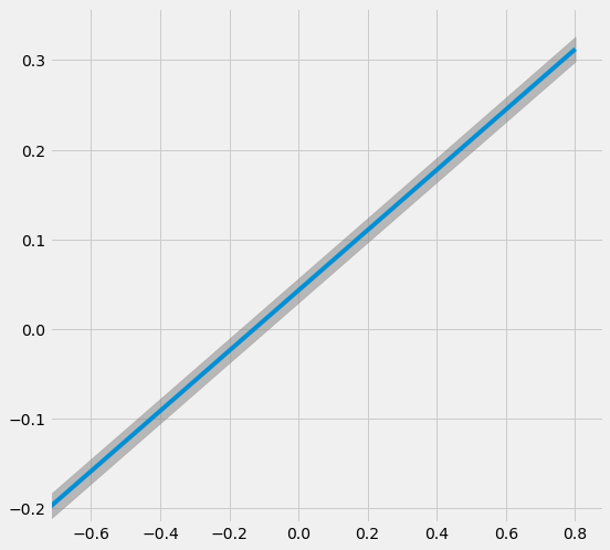
# Plot the results by confounding vector and plot Confidence Intervals for ATE
sens_x_bias_alignment.plot(lls_x_bias_alignment, ci=True)

../_images/examples_sensitivity_example_with_synthetic_data_22_0.png

[17]:

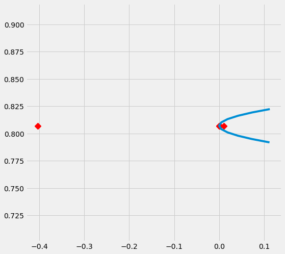
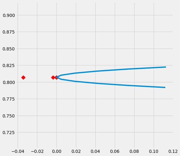
# Plot the results by rsquare with partial r-square results by each individual features
sens_x_bias_alignment.plot(lls_x_bias_alignment, partial_rsqs_x_bias_alignment, type='r.squared', partial_rsqs=True)

../_images/examples_sensitivity_example_with_synthetic_data_23_0.png

Drop One Confounder

[18]:

df_new = df.drop('feature_0', axis=1).copy()
INFERENCE_FEATURES_new = INFERENCE_FEATURES.copy()
INFERENCE_FEATURES_new.remove('feature_0')
df_new.head()

[18]:

	feature_1	feature_2	feature_3	feature_4	feature_5	target	outcome	pihat
0	0.2911	0.0432	0.8720	0.5190	0.0822	1	2.0220	0.7657
1	0.3096	0.5115	0.2048	0.8914	0.5015	0	-0.0732	0.2304
2	0.0765	0.7428	0.6951	0.4580	0.7800	0	-1.4947	0.1000
3	0.3967	0.6278	0.2086	0.3865	0.8860	0	0.6458	0.2533
4	0.0578	0.3972	0.4100	0.5760	0.4764	0	-0.0018	0.1000

[19]:

INFERENCE_FEATURES_new

[19]:

['feature_1', 'feature_2', 'feature_3', 'feature_4', 'feature_5']

Sensitivity Analysis Summary Report (with One-sided confounding function and default alpha)

[20]:

sens_x_new = Sensitivity(df=df_new, inference_features=INFERENCE_FEATURES_new, p_col='pihat',
                     treatment_col=TREATMENT_COL, outcome_col=OUTCOME_COL, learner=learner_x)
# Here for Selection Bias method will use default one-sided confounding function and alpha (quantile range of outcome values) input
sens_sumary_x_new = sens_x_new.sensitivity_analysis(methods=['Placebo Treatment',
                                                     'Random Cause',
                                                     'Subset Data',
                                                     'Random Replace',
                                                     'Selection Bias'], sample_size=0.5)

[21]:

# Here we can see the New ATE restul from Random Replace method actually changed ~ 12.5%
sens_sumary_x_new

[21]:

	Method	ATE	New ATE	New ATE LB	New ATE UB
0	Placebo Treatment	0.8072	0.0104	-0.0033	0.0242
0	Random Cause	0.8072	0.8072	0.7943	0.8201
0	Subset Data(sample size @0.5)	0.8072	0.8180	0.7998	0.8361
0	Random Replace	0.8072	0.8068	0.7938	0.8198
0	Selection Bias (alpha@-0.80111, with r-sqaure:...	0.8072	1.3799	1.3673	1.3925
0	Selection Bias (alpha@-0.64088, with r-sqaure:...	0.8072	1.2654	1.2527	1.2780
0	Selection Bias (alpha@-0.48066, with r-sqaure:...	0.8072	1.1508	1.1381	1.1635
0	Selection Bias (alpha@-0.32044, with r-sqaure:...	0.8072	1.0363	1.0235	1.0490
0	Selection Bias (alpha@-0.16022, with r-sqaure:...	0.8072	0.9217	0.9089	0.9345
0	Selection Bias (alpha@0.0, with r-sqaure:0.0	0.8072	0.8072	0.7943	0.8200
0	Selection Bias (alpha@0.16022, with r-sqaure:0...	0.8072	0.6926	0.6796	0.7056
0	Selection Bias (alpha@0.32044, with r-sqaure:0...	0.8072	0.5780	0.5650	0.5911
0	Selection Bias (alpha@0.48066, with r-sqaure:0...	0.8072	0.4635	0.4503	0.4767
0	Selection Bias (alpha@0.64088, with r-sqaure:0...	0.8072	0.3489	0.3356	0.3623
0	Selection Bias (alpha@0.80111, with r-sqaure:0...	0.8072	0.2344	0.2209	0.2479

Random Replace

[22]:

# Replace feature_0 with an irrelevent variable
sens_x_replace_new = SensitivityRandomReplace(df=df_new, inference_features=INFERENCE_FEATURES_new, p_col='pihat',
                                          treatment_col=TREATMENT_COL, outcome_col=OUTCOME_COL, learner=learner_x,
                                          sample_size=0.9, replaced_feature='feature_1')
s_check_replace_new = sens_x_replace_new.summary(method='Random Replace')
s_check_replace_new

[22]:

	Method	ATE	New ATE	New ATE LB	New ATE UB
0	Random Replace	0.8072	0.9022	0.8893	0.9152

Selection Bias: Alignment confounding Function

[23]:

sens_x_bias_alignment_new = SensitivitySelectionBias(df_new, INFERENCE_FEATURES_new, p_col='pihat', treatment_col=TREATMENT_COL,
                                                 outcome_col=OUTCOME_COL, learner=learner_x, confound='alignment',
                                                 alpha_range=None)

[24]:

lls_x_bias_alignment_new, partial_rsqs_x_bias_alignment_new = sens_x_bias_alignment_new.causalsens()

[25]:

lls_x_bias_alignment_new

[25]:

	alpha	rsqs	New ATE	New ATE LB	New ATE UB
0	-0.8011	0.1121	0.7919	0.7789	0.8049
0	-0.6409	0.0732	0.7950	0.7820	0.8079
0	-0.4807	0.0419	0.7980	0.7851	0.8109
0	-0.3204	0.0188	0.8011	0.7882	0.8139
0	-0.1602	0.0047	0.8041	0.7912	0.8170
0	0.0000	0.0000	0.8072	0.7943	0.8200
0	0.1602	0.0048	0.8102	0.7973	0.8231
0	0.3204	0.0189	0.8133	0.8003	0.8262
0	0.4807	0.0420	0.8163	0.8032	0.8294
0	0.6409	0.0736	0.8194	0.8062	0.8325
0	0.8011	0.1127	0.8224	0.8091	0.8357

[26]:

partial_rsqs_x_bias_alignment_new

[26]:

	feature	partial_rsqs
0	feature_1	-0.0345
1	feature_2	-0.0001
2	feature_3	-0.0038
3	feature_4	-0.0001
4	feature_5	0.0000

[27]:

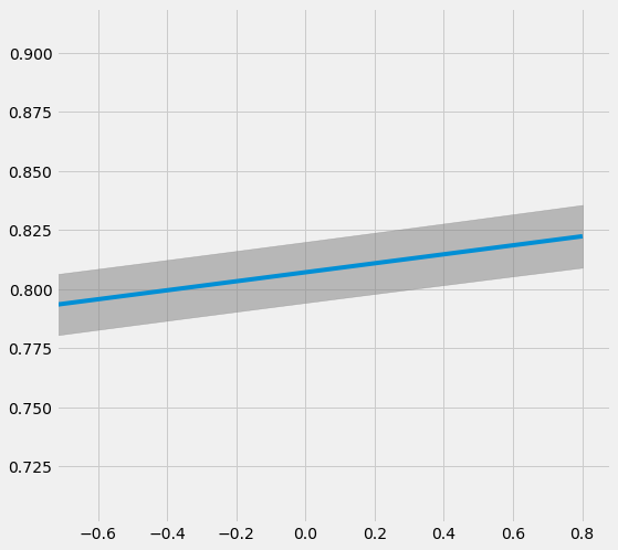
# Plot the results by confounding vector and plot Confidence Intervals for ATE
sens_x_bias_alignment_new.plot(lls_x_bias_alignment_new, ci=True)

../_images/examples_sensitivity_example_with_synthetic_data_37_0.png

[28]:

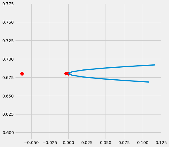
# Plot the results by rsquare with partial r-square results by each individual features
sens_x_bias_alignment_new.plot(lls_x_bias_alignment_new, partial_rsqs_x_bias_alignment_new, type='r.squared', partial_rsqs=True)

../_images/examples_sensitivity_example_with_synthetic_data_38_0.png

Generate a Selection Bias Set

[29]:

df_new_2 = df.copy()
df_new_2['treated_new'] = df['feature_0'].rank()
df_new_2['treated_new'] = [1 if i > df_new_2.shape[0]/2 else 0 for i in df_new_2['treated_new']]

[30]:

df_new_2.head()

[30]:

	feature_0	feature_1	feature_2	feature_3	feature_4	feature_5	target	outcome	pihat	treated_new
0	0.9536	0.2911	0.0432	0.8720	0.5190	0.0822	1	2.0220	0.7657	1
1	0.2390	0.3096	0.5115	0.2048	0.8914	0.5015	0	-0.0732	0.2304	0
2	0.1091	0.0765	0.7428	0.6951	0.4580	0.7800	0	-1.4947	0.1000	0
3	0.2055	0.3967	0.6278	0.2086	0.3865	0.8860	0	0.6458	0.2533	0
4	0.4501	0.0578	0.3972	0.4100	0.5760	0.4764	0	-0.0018	0.1000	0

Sensitivity Analysis Summary Report (with One-sided confounding function and default alpha)

[31]:

sens_x_new_2 = Sensitivity(df=df_new_2, inference_features=INFERENCE_FEATURES, p_col='pihat',
                     treatment_col='treated_new', outcome_col=OUTCOME_COL, learner=learner_x)
# Here for Selection Bias method will use default one-sided confounding function and alpha (quantile range of outcome values) input
sens_sumary_x_new_2 = sens_x_new_2.sensitivity_analysis(methods=['Placebo Treatment',
                                                     'Random Cause',
                                                     'Subset Data',
                                                     'Random Replace',
                                                     'Selection Bias'], sample_size=0.5)

[32]:

sens_sumary_x_new_2

[32]:

	Method	ATE	New ATE	New ATE LB	New ATE UB
0	Placebo Treatment	0.0432	0.0081	-0.0052	0.0213
0	Random Cause	0.0432	0.0432	0.0296	0.0568
0	Subset Data(sample size @0.5)	0.0432	0.0976	0.0784	0.1167
0	Random Replace	0.0432	0.0433	0.0297	0.0568
0	Selection Bias (alpha@-0.80111, with r-sqaure:...	0.0432	0.8369	0.8239	0.8499
0	Selection Bias (alpha@-0.64088, with r-sqaure:...	0.0432	0.6782	0.6651	0.6913
0	Selection Bias (alpha@-0.48066, with r-sqaure:...	0.0432	0.5194	0.5063	0.5326
0	Selection Bias (alpha@-0.32044, with r-sqaure:...	0.0432	0.3607	0.3474	0.3740
0	Selection Bias (alpha@-0.16022, with r-sqaure:...	0.0432	0.2020	0.1885	0.2154
0	Selection Bias (alpha@0.0, with r-sqaure:0.0	0.0432	0.0432	0.0296	0.0568
0	Selection Bias (alpha@0.16022, with r-sqaure:0...	0.0432	-0.1155	-0.1293	-0.1018
0	Selection Bias (alpha@0.32044, with r-sqaure:0...	0.0432	-0.2743	-0.2882	-0.2604
0	Selection Bias (alpha@0.48066, with r-sqaure:0...	0.0432	-0.4330	-0.4471	-0.4189
0	Selection Bias (alpha@0.64088, with r-sqaure:0...	0.0432	-0.5918	-0.6060	-0.5775
0	Selection Bias (alpha@0.80111, with r-sqaure:0...	0.0432	-0.7505	-0.7650	-0.7360

Random Replace

[33]:

# Replace feature_0 with an irrelevent variable
sens_x_replace_new_2 = SensitivityRandomReplace(df=df_new_2, inference_features=INFERENCE_FEATURES, p_col='pihat',
                                          treatment_col='treated_new', outcome_col=OUTCOME_COL, learner=learner_x,
                                          sample_size=0.9, replaced_feature='feature_0')
s_check_replace_new_2 = sens_x_replace_new_2.summary(method='Random Replace')
s_check_replace_new_2

[33]:

	Method	ATE	New ATE	New ATE LB	New ATE UB
0	Random Replace	0.0432	0.4847	0.4713	0.4981

Selection Bias: Alignment confounding Function

[34]:

sens_x_bias_alignment_new_2 = SensitivitySelectionBias(df_new_2, INFERENCE_FEATURES, p_col='pihat', treatment_col='treated_new',
                                                 outcome_col=OUTCOME_COL, learner=learner_x, confound='alignment',
                                                 alpha_range=None)

[35]:

lls_x_bias_alignment_new_2, partial_rsqs_x_bias_alignment_new_2 = sens_x_bias_alignment_new_2.causalsens()

[36]:

lls_x_bias_alignment_new_2

[36]:

	alpha	rsqs	New ATE	New ATE LB	New ATE UB
0	-0.8011	0.0604	-0.2260	-0.2399	-0.2120
0	-0.6409	0.0415	-0.1721	-0.1860	-0.1583
0	-0.4807	0.0250	-0.1183	-0.1320	-0.1045
0	-0.3204	0.0119	-0.0645	-0.0781	-0.0508
0	-0.1602	0.0032	-0.0106	-0.0242	0.0030
0	0.0000	0.0000	0.0432	0.0296	0.0568
0	0.1602	0.0035	0.0971	0.0835	0.1106
0	0.3204	0.0148	0.1509	0.1373	0.1645
0	0.4807	0.0347	0.2047	0.1911	0.2183
0	0.6409	0.0635	0.2586	0.2449	0.2722
0	0.8011	0.1013	0.3124	0.2986	0.3262

[37]:

partial_rsqs_x_bias_alignment_new_2

[37]:

	feature	partial_rsqs
0	feature_0	-0.4041
1	feature_1	0.0101
2	feature_2	0.0000
3	feature_3	0.0016
4	feature_4	0.0011
5	feature_5	0.0000

[38]:

# Plot the results by confounding vector and plot Confidence Intervals for ATE
sens_x_bias_alignment_new_2.plot(lls_x_bias_alignment_new_2, ci=True)

../_images/examples_sensitivity_example_with_synthetic_data_52_0.png

[39]:

# Plot the results by rsquare with partial r-square results by each individual features
sens_x_bias_alignment_new_2.plot(lls_x_bias_alignment_new, partial_rsqs_x_bias_alignment_new_2, type='r.squared', partial_rsqs=True)

../_images/examples_sensitivity_example_with_synthetic_data_53_0.png

Read the Docs v: latest

Versions: latest; stable; huigang-doc_update

Downloads: pdf; html; epub

On Read the Docs: Project Home; Builds