Meta-Learners Examples - Training, Estimation, Validation, Visualization

Introduction

In this notebook, we will generate some synthetic data to demonstrate how to use the various Meta-Learner algorithms in order to estimate Individual Treatment Effects and Average Treatment Effects with confidence intervals.

%load_ext autoreload
%autoreload 2

from causalml.inference.meta import LRSRegressor

/Users/jeong/miniconda3/envs/causalml/lib/python3.8/site-packages/shap/utils/_clustering.py:35: NumbaDeprecationWarning: The 'nopython' keyword argument was not supplied to the 'numba.jit' decorator. The implicit default value for this argument is currently False, but it will be changed to True in Numba 0.59.0. See https://numba.readthedocs.io/en/stable/reference/deprecation.html#deprecation-of-object-mode-fall-back-behaviour-when-using-jit for details.
  def _pt_shuffle_rec(i, indexes, index_mask, partition_tree, M, pos):
/Users/jeong/miniconda3/envs/causalml/lib/python3.8/site-packages/shap/utils/_clustering.py:54: NumbaDeprecationWarning: The 'nopython' keyword argument was not supplied to the 'numba.jit' decorator. The implicit default value for this argument is currently False, but it will be changed to True in Numba 0.59.0. See https://numba.readthedocs.io/en/stable/reference/deprecation.html#deprecation-of-object-mode-fall-back-behaviour-when-using-jit for details.
  def delta_minimization_order(all_masks, max_swap_size=100, num_passes=2):
/Users/jeong/miniconda3/envs/causalml/lib/python3.8/site-packages/shap/utils/_clustering.py:63: NumbaDeprecationWarning: The 'nopython' keyword argument was not supplied to the 'numba.jit' decorator. The implicit default value for this argument is currently False, but it will be changed to True in Numba 0.59.0. See https://numba.readthedocs.io/en/stable/reference/deprecation.html#deprecation-of-object-mode-fall-back-behaviour-when-using-jit for details.
  def _reverse_window(order, start, length):
/Users/jeong/miniconda3/envs/causalml/lib/python3.8/site-packages/shap/utils/_clustering.py:69: NumbaDeprecationWarning: The 'nopython' keyword argument was not supplied to the 'numba.jit' decorator. The implicit default value for this argument is currently False, but it will be changed to True in Numba 0.59.0. See https://numba.readthedocs.io/en/stable/reference/deprecation.html#deprecation-of-object-mode-fall-back-behaviour-when-using-jit for details.
  def _reverse_window_score_gain(masks, order, start, length):
/Users/jeong/miniconda3/envs/causalml/lib/python3.8/site-packages/shap/utils/_clustering.py:77: NumbaDeprecationWarning: The 'nopython' keyword argument was not supplied to the 'numba.jit' decorator. The implicit default value for this argument is currently False, but it will be changed to True in Numba 0.59.0. See https://numba.readthedocs.io/en/stable/reference/deprecation.html#deprecation-of-object-mode-fall-back-behaviour-when-using-jit for details.
  def _mask_delta_score(m1, m2):
/Users/jeong/miniconda3/envs/causalml/lib/python3.8/site-packages/shap/links.py:5: NumbaDeprecationWarning: The 'nopython' keyword argument was not supplied to the 'numba.jit' decorator. The implicit default value for this argument is currently False, but it will be changed to True in Numba 0.59.0. See https://numba.readthedocs.io/en/stable/reference/deprecation.html#deprecation-of-object-mode-fall-back-behaviour-when-using-jit for details.
  def identity(x):
/Users/jeong/miniconda3/envs/causalml/lib/python3.8/site-packages/shap/links.py:10: NumbaDeprecationWarning: The 'nopython' keyword argument was not supplied to the 'numba.jit' decorator. The implicit default value for this argument is currently False, but it will be changed to True in Numba 0.59.0. See https://numba.readthedocs.io/en/stable/reference/deprecation.html#deprecation-of-object-mode-fall-back-behaviour-when-using-jit for details.
  def _identity_inverse(x):
/Users/jeong/miniconda3/envs/causalml/lib/python3.8/site-packages/shap/links.py:15: NumbaDeprecationWarning: The 'nopython' keyword argument was not supplied to the 'numba.jit' decorator. The implicit default value for this argument is currently False, but it will be changed to True in Numba 0.59.0. See https://numba.readthedocs.io/en/stable/reference/deprecation.html#deprecation-of-object-mode-fall-back-behaviour-when-using-jit for details.
  def logit(x):
/Users/jeong/miniconda3/envs/causalml/lib/python3.8/site-packages/shap/links.py:20: NumbaDeprecationWarning: The 'nopython' keyword argument was not supplied to the 'numba.jit' decorator. The implicit default value for this argument is currently False, but it will be changed to True in Numba 0.59.0. See https://numba.readthedocs.io/en/stable/reference/deprecation.html#deprecation-of-object-mode-fall-back-behaviour-when-using-jit for details.
  def _logit_inverse(x):
/Users/jeong/miniconda3/envs/causalml/lib/python3.8/site-packages/shap/utils/_masked_model.py:363: NumbaDeprecationWarning: The 'nopython' keyword argument was not supplied to the 'numba.jit' decorator. The implicit default value for this argument is currently False, but it will be changed to True in Numba 0.59.0. See https://numba.readthedocs.io/en/stable/reference/deprecation.html#deprecation-of-object-mode-fall-back-behaviour-when-using-jit for details.
  def _build_fixed_single_output(averaged_outs, last_outs, outputs, batch_positions, varying_rows, num_varying_rows, link, linearizing_weights):
/Users/jeong/miniconda3/envs/causalml/lib/python3.8/site-packages/shap/utils/_masked_model.py:385: NumbaDeprecationWarning: The 'nopython' keyword argument was not supplied to the 'numba.jit' decorator. The implicit default value for this argument is currently False, but it will be changed to True in Numba 0.59.0. See https://numba.readthedocs.io/en/stable/reference/deprecation.html#deprecation-of-object-mode-fall-back-behaviour-when-using-jit for details.
  def _build_fixed_multi_output(averaged_outs, last_outs, outputs, batch_positions, varying_rows, num_varying_rows, link, linearizing_weights):
/Users/jeong/miniconda3/envs/causalml/lib/python3.8/site-packages/shap/utils/_masked_model.py:428: NumbaDeprecationWarning: The 'nopython' keyword argument was not supplied to the 'numba.jit' decorator. The implicit default value for this argument is currently False, but it will be changed to True in Numba 0.59.0. See https://numba.readthedocs.io/en/stable/reference/deprecation.html#deprecation-of-object-mode-fall-back-behaviour-when-using-jit for details.
  def _init_masks(cluster_matrix, M, indices_row_pos, indptr):
/Users/jeong/miniconda3/envs/causalml/lib/python3.8/site-packages/shap/utils/_masked_model.py:439: NumbaDeprecationWarning: The 'nopython' keyword argument was not supplied to the 'numba.jit' decorator. The implicit default value for this argument is currently False, but it will be changed to True in Numba 0.59.0. See https://numba.readthedocs.io/en/stable/reference/deprecation.html#deprecation-of-object-mode-fall-back-behaviour-when-using-jit for details.
  def _rec_fill_masks(cluster_matrix, indices_row_pos, indptr, indices, M, ind):
/Users/jeong/miniconda3/envs/causalml/lib/python3.8/site-packages/shap/maskers/_tabular.py:186: NumbaDeprecationWarning: The 'nopython' keyword argument was not supplied to the 'numba.jit' decorator. The implicit default value for this argument is currently False, but it will be changed to True in Numba 0.59.0. See https://numba.readthedocs.io/en/stable/reference/deprecation.html#deprecation-of-object-mode-fall-back-behaviour-when-using-jit for details.
  def _single_delta_mask(dind, masked_inputs, last_mask, data, x, noop_code):
/Users/jeong/miniconda3/envs/causalml/lib/python3.8/site-packages/shap/maskers/_tabular.py:197: NumbaDeprecationWarning: The 'nopython' keyword argument was not supplied to the 'numba.jit' decorator. The implicit default value for this argument is currently False, but it will be changed to True in Numba 0.59.0. See https://numba.readthedocs.io/en/stable/reference/deprecation.html#deprecation-of-object-mode-fall-back-behaviour-when-using-jit for details.
  def _delta_masking(masks, x, curr_delta_inds, varying_rows_out,
/Users/jeong/miniconda3/envs/causalml/lib/python3.8/site-packages/tqdm/auto.py:22: TqdmWarning: IProgress not found. Please update jupyter and ipywidgets. See https://ipywidgets.readthedocs.io/en/stable/user_install.html
  from .autonotebook import tqdm as notebook_tqdm
/Users/jeong/miniconda3/envs/causalml/lib/python3.8/site-packages/shap/maskers/_image.py:175: NumbaDeprecationWarning: The 'nopython' keyword argument was not supplied to the 'numba.jit' decorator. The implicit default value for this argument is currently False, but it will be changed to True in Numba 0.59.0. See https://numba.readthedocs.io/en/stable/reference/deprecation.html#deprecation-of-object-mode-fall-back-behaviour-when-using-jit for details.
  def _jit_build_partition_tree(xmin, xmax, ymin, ymax, zmin, zmax, total_ywidth, total_zwidth, M, clustering, q):
/Users/jeong/miniconda3/envs/causalml/lib/python3.8/site-packages/shap/explainers/_partition.py:676: NumbaDeprecationWarning: The 'nopython' keyword argument was not supplied to the 'numba.jit' decorator. The implicit default value for this argument is currently False, but it will be changed to True in Numba 0.59.0. See https://numba.readthedocs.io/en/stable/reference/deprecation.html#deprecation-of-object-mode-fall-back-behaviour-when-using-jit for details.
  def lower_credit(i, value, M, values, clustering):
The 'nopython' keyword argument was not supplied to the 'numba.jit' decorator. The implicit default value for this argument is currently False, but it will be changed to True in Numba 0.59.0. See https://numba.readthedocs.io/en/stable/reference/deprecation.html#deprecation-of-object-mode-fall-back-behaviour-when-using-jit for details.
The 'nopython' keyword argument was not supplied to the 'numba.jit' decorator. The implicit default value for this argument is currently False, but it will be changed to True in Numba 0.59.0. See https://numba.readthedocs.io/en/stable/reference/deprecation.html#deprecation-of-object-mode-fall-back-behaviour-when-using-jit for details.

import pandas as pd
import numpy as np
from matplotlib import pyplot as plt
from sklearn.linear_model import LinearRegression
from sklearn.model_selection import train_test_split
import statsmodels.api as sm
from xgboost import XGBRegressor
import warnings

from causalml.inference.meta import LRSRegressor
from causalml.inference.meta import XGBTRegressor, MLPTRegressor
from causalml.inference.meta import BaseXRegressor, BaseRRegressor, BaseSRegressor, BaseTRegressor
from causalml.match import NearestNeighborMatch, MatchOptimizer, create_table_one
from causalml.propensity import ElasticNetPropensityModel
from causalml.dataset import *
from causalml.metrics import *

warnings.filterwarnings('ignore')
plt.style.use('fivethirtyeight')

%matplotlib inline

Failed to import duecredit due to No module named 'duecredit'

import importlib
print(importlib.metadata.version('causalml') )

0.15.1.dev0

Part A: Example Workflow using Synthetic Data

Generate synthetic data

• We have implemented 4 modes of generating synthetic data (specified by input parameter mode). Refer to the References section for more detail on these data generation processes.

# Generate synthetic data using mode 1
y, X, treatment, tau, b, e = synthetic_data(mode=1, n=10000, p=8, sigma=1.0)

Calculate Average Treatment Effect (ATE)

A meta-learner can be instantiated by calling a base learner class and providing an sklearn/xgboost regressor class as input. Alternatively, we have provided some ready-to-use learners that have already inherited their respective base learner class capabilities. This is more abstracted and allows these tools to be quickly and readily usable.

# Ready-to-use S-Learner using LinearRegression
learner_s = LRSRegressor()
ate_s = learner_s.estimate_ate(X=X, treatment=treatment, y=y)
print(ate_s)
print('ATE estimate: {:.03f}'.format(ate_s[0][0]))
print('ATE lower bound: {:.03f}'.format(ate_s[1][0]))
print('ATE upper bound: {:.03f}'.format(ate_s[2][0]))

# After calling estimate_ate, add pretrain=True flag to skip training
# This flag is applicable for other meta learner
ate_s = learner_s.estimate_ate(X=X, treatment=treatment, y=y, pretrain=True)
print(ate_s)
print('ATE estimate: {:.03f}'.format(ate_s[0][0]))
print('ATE lower bound: {:.03f}'.format(ate_s[1][0]))
print('ATE upper bound: {:.03f}'.format(ate_s[2][0]))

(array([0.72721128]), array([0.67972656]), array([0.77469599]))
ATE estimate: 0.727
ATE lower bound: 0.680
ATE upper bound: 0.775
(array([0.72721128]), array([0.67972656]), array([0.77469599]))
ATE estimate: 0.727
ATE lower bound: 0.680
ATE upper bound: 0.775

# Ready-to-use T-Learner using XGB
learner_t = XGBTRegressor()
ate_t = learner_t.estimate_ate(X=X, treatment=treatment, y=y)
print('Using the ready-to-use XGBTRegressor class')
print(ate_t)

# Calling the Base Learner class and feeding in XGB
learner_t = BaseTRegressor(learner=XGBRegressor())
ate_t = learner_t.estimate_ate(X=X, treatment=treatment, y=y)
print('\nUsing the BaseTRegressor class and using XGB (same result):')
print(ate_t)

# Calling the Base Learner class and feeding in LinearRegression
learner_t = BaseTRegressor(learner=LinearRegression())
ate_t = learner_t.estimate_ate(X=X, treatment=treatment, y=y)
print('\nUsing the BaseTRegressor class and using Linear Regression (different result):')
print(ate_t)

Using the ready-to-use XGBTRegressor class
(array([0.55539207]), array([0.53185148]), array([0.57893267]))

Using the BaseTRegressor class and using XGB (same result):
(array([0.55539207]), array([0.53185148]), array([0.57893267]))

Using the BaseTRegressor class and using Linear Regression (different result):
(array([0.71740976]), array([0.67655445]), array([0.75826507]))

# X Learner with propensity score input
# Calling the Base Learner class and feeding in XGB
learner_x = BaseXRegressor(learner=XGBRegressor())
ate_x = learner_x.estimate_ate(X=X, treatment=treatment, y=y, p=e)
print('Using the BaseXRegressor class and using XGB:')
print(ate_x)

# Calling the Base Learner class and feeding in LinearRegression
learner_x = BaseXRegressor(learner=LinearRegression())
ate_x = learner_x.estimate_ate(X=X, treatment=treatment, y=y, p=e)
print('\nUsing the BaseXRegressor class and using Linear Regression:')
print(ate_x)

Using the BaseXRegressor class and using XGB:
(array([0.52239345]), array([0.50279387]), array([0.54199302]))

Using the BaseXRegressor class and using Linear Regression:
(array([0.71740976]), array([0.67655445]), array([0.75826507]))

# X Learner without propensity score input
# Calling the Base Learner class and feeding in XGB
learner_x = BaseXRegressor(XGBRegressor())
ate_x = learner_x.estimate_ate(X=X, treatment=treatment, y=y)
print('Using the BaseXRegressor class and using XGB without propensity score input:')
print(ate_x)

# Calling the Base Learner class and feeding in LinearRegression
learner_x = BaseXRegressor(learner=LinearRegression())
ate_x = learner_x.estimate_ate(X=X, treatment=treatment, y=y)
print('\nUsing the BaseXRegressor class and using Linear Regression without propensity score input:')
print(ate_x)

Using the BaseXRegressor class and using XGB without propensity score input:
(array([0.52348025]), array([0.50385245]), array([0.54310804]))

Using the BaseXRegressor class and using Linear Regression without propensity score input:
(array([0.71740976]), array([0.67655445]), array([0.75826507]))

# R Learner with propensity score input
# Calling the Base Learner class and feeding in XGB
learner_r = BaseRRegressor(learner=XGBRegressor())
ate_r = learner_r.estimate_ate(X=X, treatment=treatment, y=y, p=e)
print('Using the BaseRRegressor class and using XGB:')
print(ate_r)

# Calling the Base Learner class and feeding in LinearRegression
learner_r = BaseRRegressor(learner=LinearRegression())
ate_r = learner_r.estimate_ate(X=X, treatment=treatment, y=y, p=e)
print('Using the BaseRRegressor class and using Linear Regression:')
print(ate_r)

Using the BaseRRegressor class and using XGB:
(array([0.51551318]), array([0.5150305]), array([0.51599587]))
Using the BaseRRegressor class and using Linear Regression:
(array([0.51503495]), array([0.51461987]), array([0.51545004]))

# R Learner with propensity score input and random sample weight
# Calling the Base Learner class and feeding in XGB
learner_r = BaseRRegressor(learner=XGBRegressor())
sample_weight = np.random.randint(1, 3, len(y))
ate_r = learner_r.estimate_ate(X=X, treatment=treatment, y=y, p=e, sample_weight=sample_weight)
print('Using the BaseRRegressor class and using XGB:')
print(ate_r)

Using the BaseRRegressor class and using XGB:
(array([0.48910448]), array([0.48861819]), array([0.48959077]))

# R Learner without propensity score input
# Calling the Base Learner class and feeding in XGB
learner_r = BaseRRegressor(learner=XGBRegressor())
ate_r = learner_r.estimate_ate(X=X, treatment=treatment, y=y)
print('Using the BaseRRegressor class and using XGB without propensity score input:')
print(ate_r)

# Calling the Base Learner class and feeding in LinearRegression
learner_r = BaseRRegressor(learner=LinearRegression())
ate_r = learner_r.estimate_ate(X=X, treatment=treatment, y=y)
print('Using the BaseRRegressor class and using Linear Regression without propensity score input:')
print(ate_r)

Using the BaseRRegressor class and using XGB without propensity score input:
(array([0.45400543]), array([0.45352042]), array([0.45449043]))
Using the BaseRRegressor class and using Linear Regression without propensity score input:
(array([0.59802659]), array([0.59761147]), array([0.5984417]))

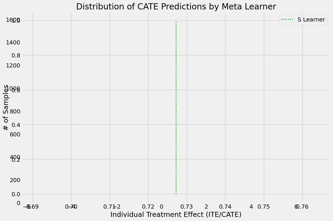
7. Calculate Individual Treatment Effect (ITE/CATE)

CATE stands for Conditional Average Treatment Effect.

# S Learner
learner_s = LRSRegressor()
cate_s = learner_s.fit_predict(X=X, treatment=treatment, y=y)

# T Learner
learner_t = BaseTRegressor(learner=XGBRegressor())
cate_t = learner_t.fit_predict(X=X, treatment=treatment, y=y)

# X Learner with propensity score input
learner_x = BaseXRegressor(learner=XGBRegressor())
cate_x = learner_x.fit_predict(X=X, treatment=treatment, y=y, p=e)

# X Learner without propensity score input
learner_x_no_p = BaseXRegressor(learner=XGBRegressor())
cate_x_no_p = learner_x_no_p.fit_predict(X=X, treatment=treatment, y=y)

# R Learner with propensity score input
learner_r = BaseRRegressor(learner=XGBRegressor())
cate_r = learner_r.fit_predict(X=X, treatment=treatment, y=y, p=e)

# R Learner without propensity score input
learner_r_no_p = BaseRRegressor(learner=XGBRegressor())
cate_r_no_p = learner_r_no_p.fit_predict(X=X, treatment=treatment, y=y)

alpha=0.2
bins=30
plt.figure(figsize=(12,8))
plt.hist(cate_t, alpha=alpha, bins=bins, label='T Learner')
plt.hist(cate_x, alpha=alpha, bins=bins, label='X Learner')
plt.hist(cate_x_no_p, alpha=alpha, bins=bins, label='X Learner (no propensity score)')
plt.hist(cate_r, alpha=alpha, bins=bins, label='R Learner')
plt.hist(cate_r_no_p, alpha=alpha, bins=bins, label='R Learner (no propensity score)')
plt.vlines(cate_s[0], 0, plt.axes().get_ylim()[1], label='S Learner',
           linestyles='dotted', colors='green', linewidth=2)
plt.title('Distribution of CATE Predictions by Meta Learner')
plt.xlabel('Individual Treatment Effect (ITE/CATE)')
plt.ylabel('# of Samples')
_=plt.legend()

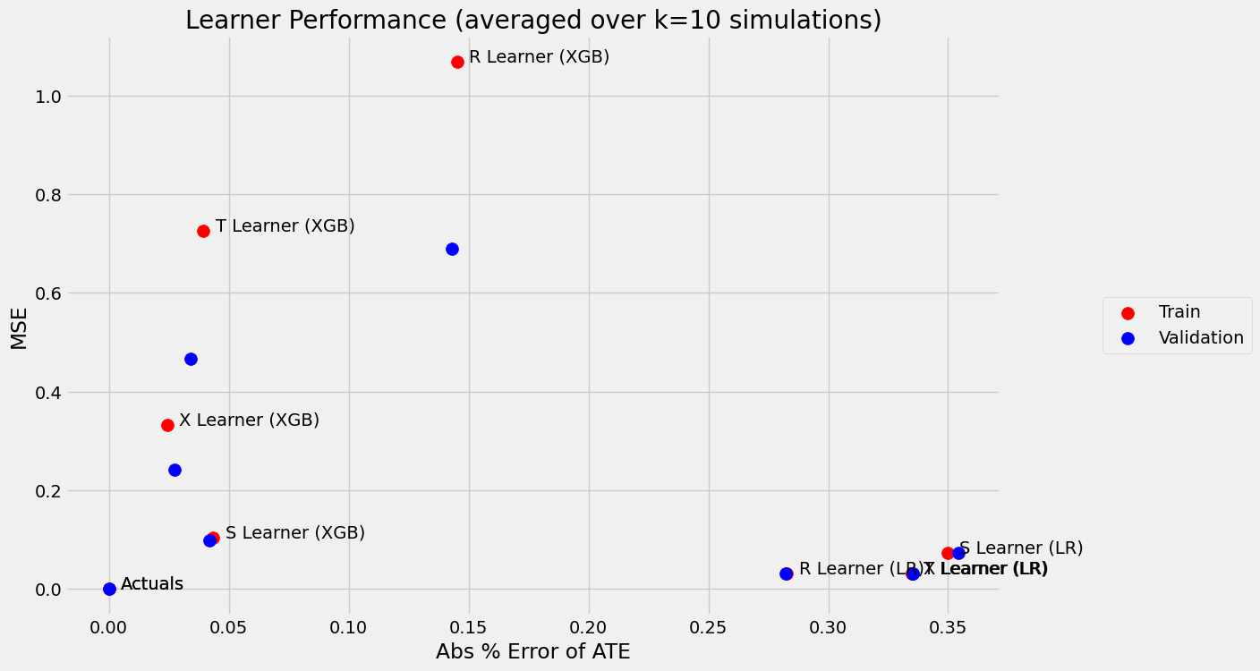
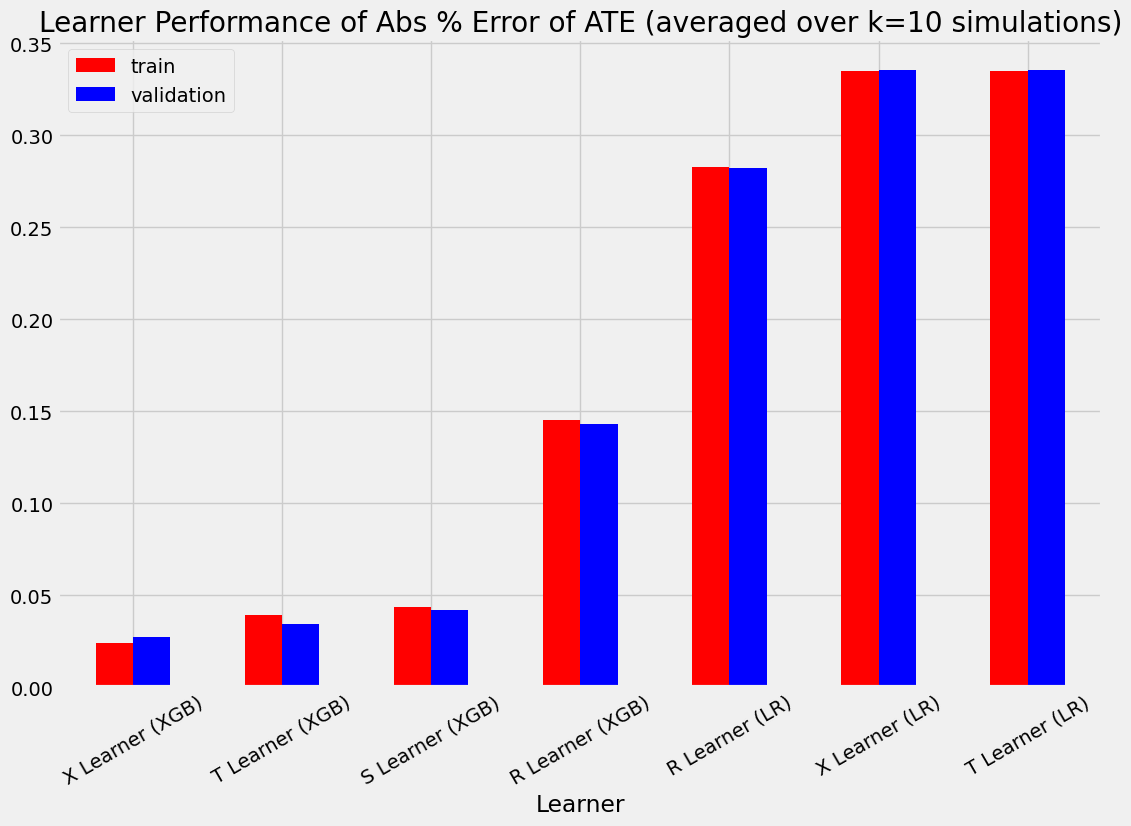
Part B: Validating Meta-Learner Accuracy

We will validate the meta-learners’ performance based on the same synthetic data generation method in Part A (simulate_nuisance_and_easy_treatment).

train_summary, validation_summary = get_synthetic_summary_holdout(simulate_nuisance_and_easy_treatment,
                                                                  n=10000,
                                                                  valid_size=0.2,
                                                                  k=10)

train_summary

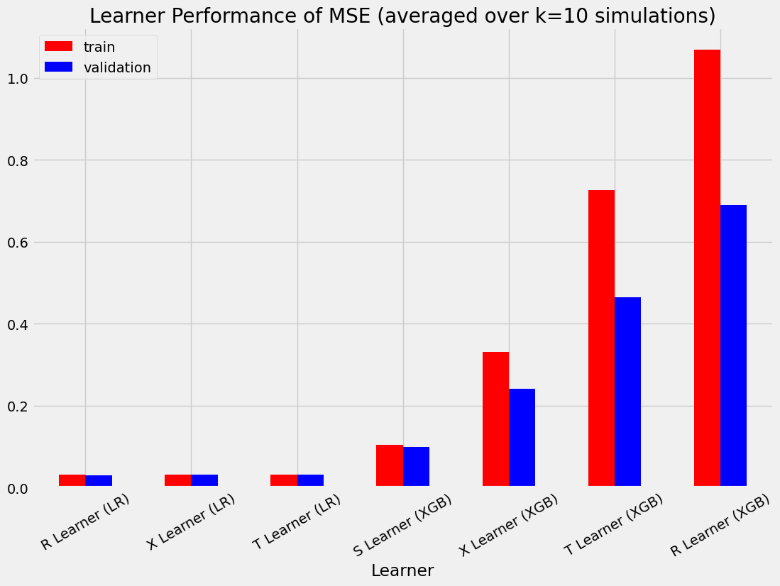
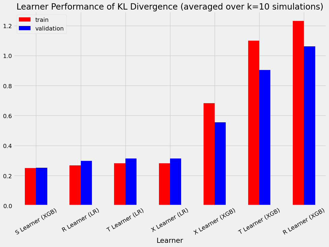
	Abs % Error of ATE	MSE	KL Divergence
Actuals	0.000000	0.000000	0.000000
S Learner (LR)	0.349749	0.072543	3.703728
S Learner (XGB)	0.043545	0.103968	0.249110
T Learner (LR)	0.334790	0.031673	0.282270
T Learner (XGB)	0.039432	0.726171	1.099338
X Learner (LR)	0.334790	0.031673	0.282270
X Learner (XGB)	0.024209	0.331760	0.682191
R Learner (LR)	0.282719	0.031079	0.267950
R Learner (XGB)	0.145131	1.068164	1.230508

validation_summary

	Abs % Error of ATE	MSE	KL Divergence
Actuals	0.000000	0.000000	0.000000
S Learner (LR)	0.354242	0.072989	3.797245
S Learner (XGB)	0.041916	0.098853	0.251344
T Learner (LR)	0.335444	0.031613	0.314690
T Learner (XGB)	0.034209	0.465331	0.904251
X Learner (LR)	0.335444	0.031613	0.314690
X Learner (XGB)	0.027473	0.241996	0.554173
R Learner (LR)	0.282196	0.030891	0.298666
R Learner (XGB)	0.143055	0.689088	1.061381

scatter_plot_summary_holdout(train_summary,
                             validation_summary,
                             k=10,
                             label=['Train', 'Validation'],
                             drop_learners=[],
                             drop_cols=[])

bar_plot_summary_holdout(train_summary,
                         validation_summary,
                         k=10,
                         drop_learners=['S Learner (LR)'],
                         drop_cols=[])

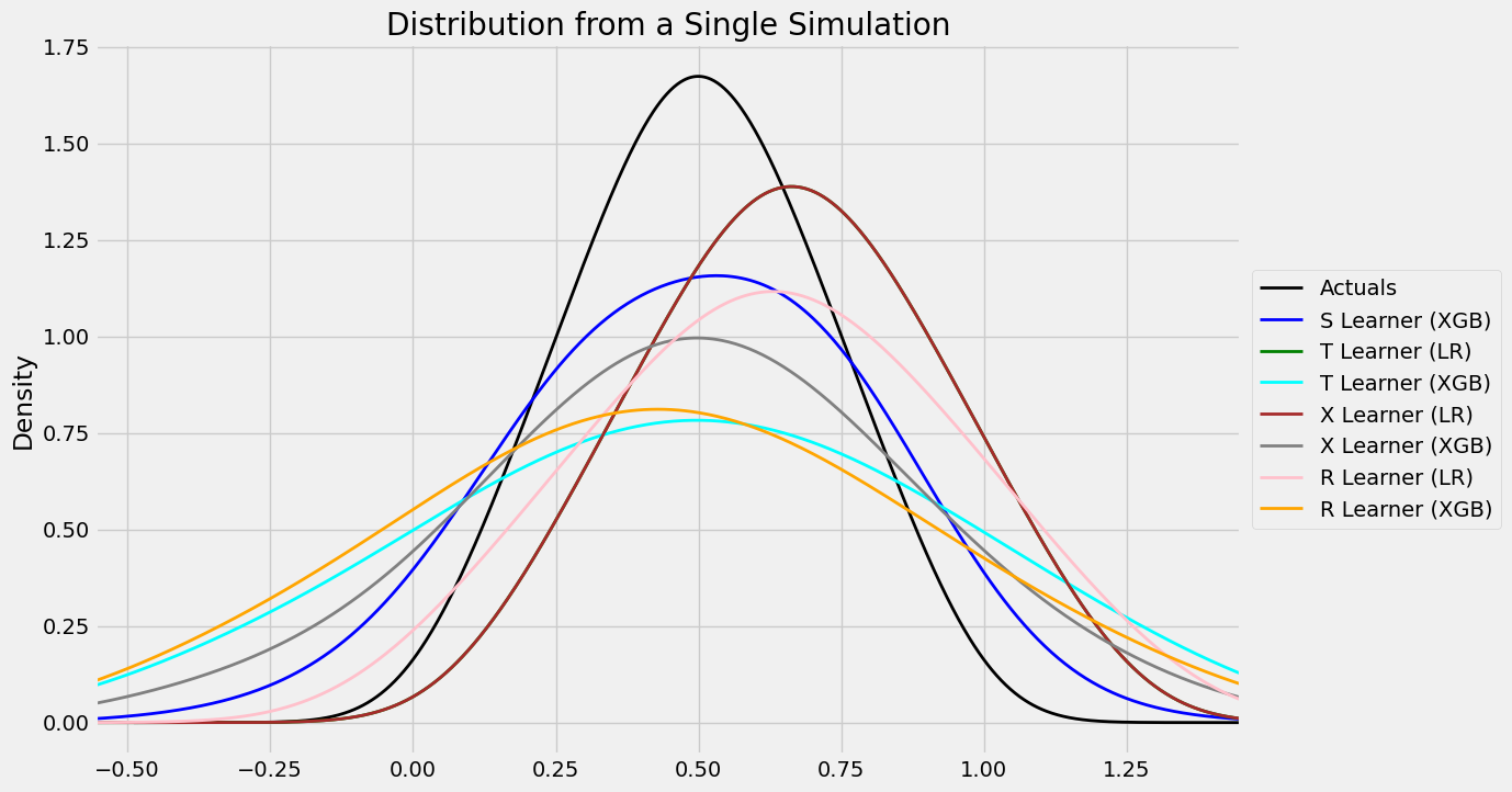
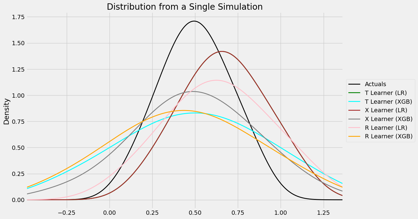
# Single simulation
train_preds, valid_preds = get_synthetic_preds_holdout(simulate_nuisance_and_easy_treatment,
                                                       n=50000,
                                                       valid_size=0.2)

#distribution plot for signle simulation of Training
distr_plot_single_sim(train_preds, kind='kde', linewidth=2, bw_method=0.5,
                      drop_learners=['S Learner (LR)',' S Learner (XGB)'])

#distribution plot for signle simulation of Validaiton
distr_plot_single_sim(valid_preds, kind='kde', linewidth=2, bw_method=0.5,
                      drop_learners=['S Learner (LR)', 'S Learner (XGB)'])

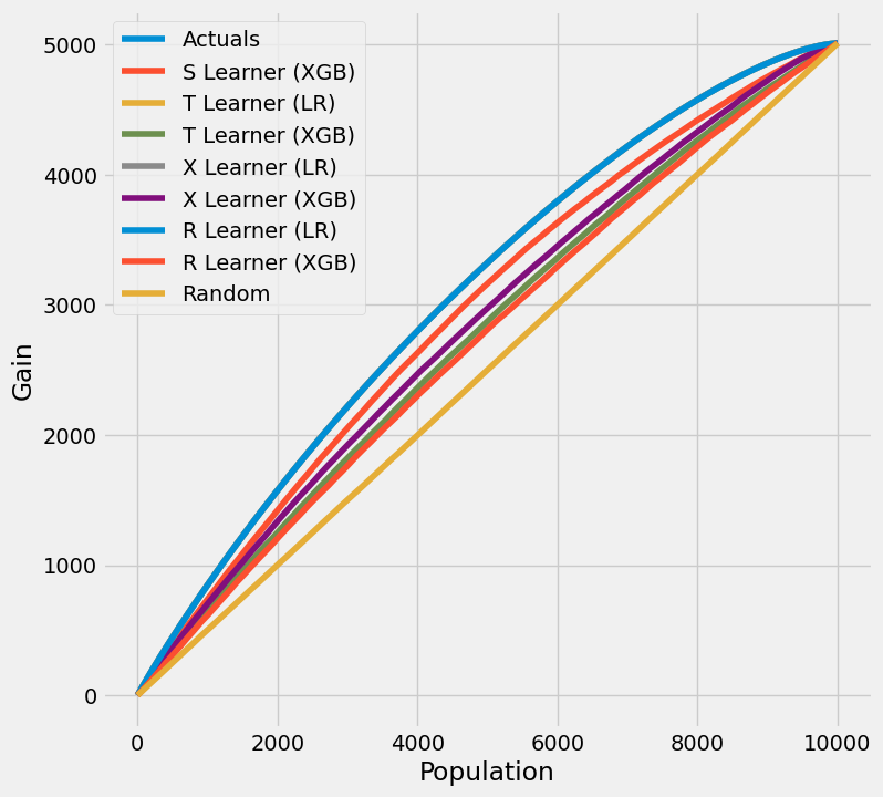
# Scatter Plots for a Single Simulation of Training Data
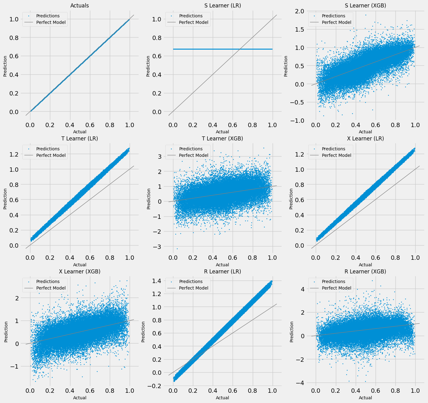
scatter_plot_single_sim(train_preds)

# Scatter Plots for a Single Simulation of Validaiton Data
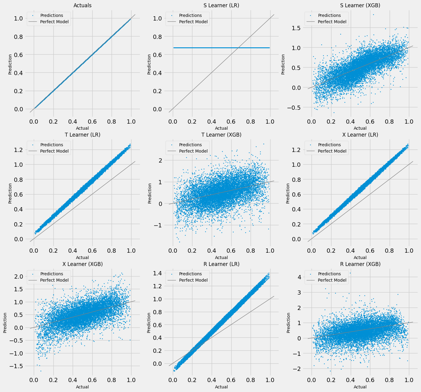
scatter_plot_single_sim(valid_preds)

# Cumulative Gain AUUC values for a Single Simulation of Training Data
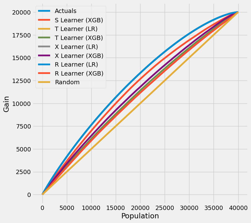
get_synthetic_auuc(train_preds, drop_learners=['S Learner (LR)'])

	Learner	cum_gain_auuc
0	Actuals	4.934321e+06
2	T Learner (LR)	4.932595e+06
4	X Learner (LR)	4.932595e+06
6	R Learner (LR)	4.931463e+06
1	S Learner (XGB)	4.707889e+06
5	X Learner (XGB)	4.507384e+06
3	T Learner (XGB)	4.389641e+06
7	R Learner (XGB)	4.309501e+06
8	Random	4.002357e+06

# Cumulative Gain AUUC values for a Single Simulation of Validaiton Data
get_synthetic_auuc(valid_preds, drop_learners=['S Learner (LR)'])

	Learner	cum_gain_auuc
0	Actuals	308122.561368
2	T Learner (LR)	308013.995722
4	X Learner (LR)	308013.995722
6	R Learner (LR)	307941.890461
1	S Learner (XGB)	294216.363545
5	X Learner (XGB)	283752.122952
3	T Learner (XGB)	276230.885568
7	R Learner (XGB)	271316.357530
8	Random	250262.193393