CEVAE: JAX vs PyTorch Backend Benchmark

This notebook compares the two CEVAE (Causal Effect Variational Autoencoder, Louizos et al. 2017) backends available in CausalML:

• causalml.inference.torch.CEVAE — the original PyTorch/pyro implementation (wraps pyro.contrib.cevae)

• causalml.inference.jax.CEVAE — the JAX/`flax.nnx <https://flax.readthedocs.io/en/latest/nnx/index.html>`__ implementation (see causalml/inference/jax/cevae/)

Both models are trained with identical hyperparameters on the same synthetic dataset with a hidden confounder, and compared on ATE, MAE (against the true ITE), AUUC, and wall-clock training time.

Requires the optional dependencies: pip install "causalml[jax,torch]".

# Avoid OMP/threading conflicts when torch and JAX share a single process on macOS.
import logging
import os
import warnings

os.environ.setdefault("KMP_DUPLICATE_LIB_OK", "TRUE")
os.environ.setdefault("OMP_NUM_THREADS", "1")

warnings.filterwarnings("ignore")

import time

import numpy as np
import pandas as pd
import torch
import pyro
from matplotlib import pyplot as plt
import seaborn as sns

from sklearn.model_selection import train_test_split
from sklearn.metrics import mean_absolute_error

from causalml.dataset import simulate_hidden_confounder
from causalml.inference.torch import CEVAE as CEVAETorch
from causalml.inference.jax import CEVAE as CEVAEJax
from causalml.metrics import auuc_score, plot_gain

# causalml.inference.torch enables DEBUG logging for pyro at import time; quiet it.
logging.getLogger("pyro").setLevel(logging.WARNING)

plt.style.use("fivethirtyeight")
sns.set_palette("Paired")
plt.rcParams["figure.figsize"] = (12, 8)

Synthetic data with a hidden confounder

simulate_hidden_confounder generates data where a latent variable biases both treatment assignment and outcome — the setting CEVAE was designed for. The ground-truth individual treatment effect tau is known, so we can score each backend directly against it.

np.random.seed(123)

y, X, w, tau, b, e = simulate_hidden_confounder(n=20000, p=5, sigma=1.0, adj=0.0)

(
    X_train,
    X_val,
    y_train,
    y_val,
    w_train,
    w_val,
    tau_train,
    tau_val,
) = train_test_split(X, y, w, tau, test_size=0.2, random_state=123, shuffle=True)

print(f"train: {X_train.shape[0]} rows | validation: {X_val.shape[0]} rows")
print(f"true ATE (train): {tau_train.mean():.4f} | true ATE (val): {tau_val.mean():.4f}")

train: 16000 rows | validation: 4000 rows
true ATE (train): 0.7293 | true ATE (val): 0.7234

Shared hyperparameters

Both backends expose the same sklearn-style API and are configured identically, so any difference in the results comes from the implementations themselves.

common = dict(
    outcome_dist="normal",
    latent_dim=20,
    hidden_dim=200,
    num_epochs=25,
    batch_size=1000,
    learning_rate=1e-3,
    learning_rate_decay=0.1,
    num_layers=3,
    num_samples=100,
)

PyTorch (pyro) backend

pyro.set_rng_seed(0)
torch.manual_seed(0)

torch_cevae = CEVAETorch(**common)

t0 = time.perf_counter()
torch_cevae.fit(
    X=torch.tensor(X_train, dtype=torch.float),
    treatment=torch.tensor(w_train, dtype=torch.float),
    y=torch.tensor(y_train, dtype=torch.float),
)
torch_time = time.perf_counter() - t0

ite_torch_train = torch_cevae.predict(X_train).ravel()
ite_torch_val = torch_cevae.predict(X_val).ravel()

print(f"PyTorch backend trained in {torch_time:.1f}s")

PyTorch backend trained in 6.7s

JAX (flax.nnx) backend

jax_cevae = CEVAEJax(**common, seed=0)

t0 = time.perf_counter()
jax_cevae.fit(X_train, w_train, y_train)
jax_time = time.perf_counter() - t0

ite_jax_train = jax_cevae.predict(X_train).ravel()
ite_jax_val = jax_cevae.predict(X_val).ravel()

print(f"JAX backend trained in {jax_time:.1f}s")

JAX backend trained in 4.6s

Benchmark results

Training set

df_preds_train = pd.DataFrame(
    [ite_torch_train, ite_jax_train, tau_train, w_train, y_train],
    index=["CEVAE (PyTorch)", "CEVAE (JAX)", "tau", "w", "y"],
).T

summary_train = pd.DataFrame(
    {
        "CEVAE (PyTorch)": [
            ite_torch_train.mean(),
            mean_absolute_error(tau_train, ite_torch_train),
            torch_time,
        ],
        "CEVAE (JAX)": [
            ite_jax_train.mean(),
            mean_absolute_error(tau_train, ite_jax_train),
            jax_time,
        ],
        "actual": [tau_train.mean(), np.nan, np.nan],
    },
    index=["ATE", "MAE", "fit time (s)"],
).T
summary_train["AUUC"] = auuc_score(df_preds_train)

summary_train

	ATE	MAE	fit time (s)	AUUC
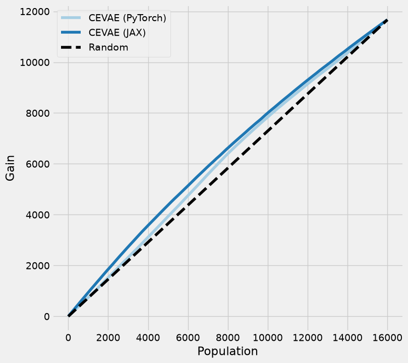
CEVAE (PyTorch)	0.884192	0.210640	6.747957	0.524815
CEVAE (JAX)	0.831832	0.205091	4.628406	0.545208
actual	0.729305	NaN	NaN	NaN

plot_gain(df_preds_train)

Validation set

df_preds_val = pd.DataFrame(
    [ite_torch_val, ite_jax_val, tau_val, w_val, y_val],
    index=["CEVAE (PyTorch)", "CEVAE (JAX)", "tau", "w", "y"],
).T

summary_val = pd.DataFrame(
    {
        "CEVAE (PyTorch)": [
            ite_torch_val.mean(),
            mean_absolute_error(tau_val, ite_torch_val),
        ],
        "CEVAE (JAX)": [
            ite_jax_val.mean(),
            mean_absolute_error(tau_val, ite_jax_val),
        ],
        "actual": [tau_val.mean(), np.nan],
    },
    index=["ATE", "MAE"],
).T
summary_val["AUUC"] = auuc_score(df_preds_val)

summary_val

	ATE	MAE	AUUC
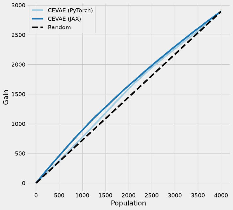
CEVAE (PyTorch)	0.884965	0.215583	0.524284
CEVAE (JAX)	0.831255	0.208282	0.545295
actual	0.723394	NaN	NaN

plot_gain(df_preds_val)

ITE distribution

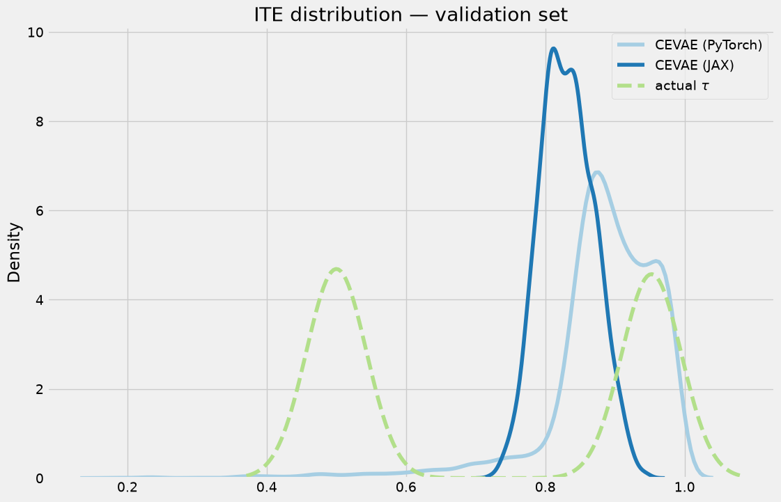
fig, ax = plt.subplots()
sns.kdeplot(ite_torch_val, label="CEVAE (PyTorch)", ax=ax)
sns.kdeplot(ite_jax_val, label="CEVAE (JAX)", ax=ax)
sns.kdeplot(tau_val, label="actual $\\tau$", ax=ax, linestyle="--")
ax.set_title("ITE distribution — validation set")
ax.legend()
plt.show()

Takeaways

• Both backends recover a comparable ATE and reach similar MAE/AUUC against the true ITE, confirming that the JAX/flax.nnx port is faithful to the reference PyTorch/pyro implementation.

• The JAX backend exposes the same sklearn-style API (fit, predict, fit_predict, save, load) and is installed via the opt-in causalml[jax] extra, so it slots into JAX-based stacks without pulling in PyTorch/pyro.