DragonNet: JAX vs TF Benchmark

Compares the JAX (flax.nnx) and TF (Keras) DragonNet implementations on the IHDP semi-synthetic dataset using ATE, MAE, AUUC, and wall-clock training time.

Reference: Shi, Blei & Veitch (2019) — https://arxiv.org/pdf/1906.02120.pdf

Setup

TF backend:

pip install tensorflow

JAX backend:

pip install "causalml[jax]"
# or: uv pip install jax flax optax orbax-checkpoint

%load_ext autoreload
%autoreload 2

import os
import time
import warnings

import numpy as np
import pandas as pd
import seaborn as sns
from matplotlib import pyplot as plt
from sklearn.metrics import mean_absolute_error

from causalml.metrics import auuc_score, plot_gain

# fmt: off
%matplotlib inline
warnings.filterwarnings("ignore")
plt.style.use("fivethirtyeight")
sns.set_palette("Paired")
plt.rcParams["figure.figsize"] = (12, 8)
# fmt: on

try:
    from causalml.inference.tf import DragonNet as TFDragonNet

    HAS_TF = True
except ImportError:
    HAS_TF = False
    print("[INFO] tensorflow not installed — TF DragonNet will be skipped.")

try:
    from causalml.inference.jax import DragonNet as JAXDragonNet

    HAS_JAX = True
except ImportError:
    HAS_JAX = False
    print("[INFO] jax/flax not installed — JAX DragonNet will be skipped.")

IHDP Dataset

Semi-synthetic dataset from Hill (2011), used in the original DragonNet paper. 747 observations from the Infant Health and Development Program (IHDP) study. We use one realisation (ihdp_npci_3.csv) to reproduce the notebook benchmark.

DATA_PATH = os.path.join(os.path.dirname(os.path.abspath("__file__")), "data", "ihdp_npci_3.csv")

df = pd.read_csv(DATA_PATH, header=None)
cols = ["treatment", "y_factual", "y_cfactual", "mu0", "mu1"] + [
    f"x{i}" for i in range(1, 26)
]
df.columns = cols

X = df.loc[:, "x1":].values
treatment = df["treatment"].values
y = df["y_factual"].values
tau = df.apply(
    lambda d: d["y_factual"] - d["y_cfactual"]
    if d["treatment"] == 1
    else d["y_cfactual"] - d["y_factual"],
    axis=1,
).values

print(f"n={len(y)},  actual ATE = {tau.mean():.4f}")
df.head()

n=747,  actual ATE = 4.0989

	treatment	y_factual	y_cfactual	mu0	mu1	x1	x2	x3	x4	x5	...	x16	x17	x18	x19	x20	x21	x22	x23	x24	x25
0	1	5.931652	3.500591	2.253801	7.136441	-0.528603	-0.343455	1.128554	0.161703	-0.316603	...	1	1	1	1	0	0	0	0	0	0
1	0	2.175966	5.952101	1.257592	6.553022	-1.736945	-1.802002	0.383828	2.244320	-0.629189	...	1	1	1	1	0	0	0	0	0	0
2	0	2.180294	7.175734	2.384100	7.192645	-0.807451	-0.202946	-0.360898	-0.879606	0.808706	...	1	0	1	1	0	0	0	0	0	0
3	0	3.587662	7.787537	4.009365	7.712456	0.390083	0.596582	-1.850350	-0.879606	-0.004017	...	1	0	1	1	0	0	0	0	0	0
4	0	2.372618	5.461871	2.481631	7.232739	-1.045229	-0.602710	0.011465	0.161703	0.683672	...	1	1	1	1	0	0	0	0	0	0

5 rows × 30 columns

Train DragonNet

SEED = 42
HYPERPARAMS = dict(neurons_per_layer=200, targeted_reg=True, verbose=False)

np.random.seed(SEED)

results = {}  # label -> {"ite": array, "train_time": float}

for label, cls, available in [
    ("TF DragonNet", TFDragonNet if HAS_TF else None, HAS_TF),
    ("JAX DragonNet", JAXDragonNet if HAS_JAX else None, HAS_JAX),
]:
    if not available:
        print(f"[{label}] skipped (backend not installed).")
        continue
    print(f"[{label}] fitting...")
    model = cls(**HYPERPARAMS)
    t0 = time.perf_counter()
    model.fit(X, treatment, y)
    train_time = time.perf_counter() - t0
    ite = model.predict_tau(X).ravel()
    results[label] = {"ite": ite, "train_time": train_time}
    print(f"[{label}] done — ATE={ite.mean():.4f},  train time={train_time:.2f}s")

[TF DragonNet] fitting...
24/24 ━━━━━━━━━━━━━━━━━━━━ 0s 1ms/step
[TF DragonNet] done — ATE=3.9952,  train time=4.42s
[JAX DragonNet] fitting...
[JAX DragonNet] done — ATE=3.9220,  train time=1.71s

Results

# Build df_preds following the same convention as dragonnet_example.ipynb:
# model columns + reserved columns tau / w / y
preds_data = {label: v["ite"] for label, v in results.items()}
preds_data.update({"tau": tau, "w": treatment, "y": y})
df_preds = pd.DataFrame(preds_data)

rows = []
for label, v in results.items():
    ite = v["ite"]
    rows.append(
        {
            "ATE": float(ite.mean()),
            "Actual ATE": float(tau.mean()),
            "MAE": float(mean_absolute_error(tau, ite)),
            "Train time (s)": float(v["train_time"]),
        }
    )

df_result = pd.DataFrame(rows, index=list(results.keys()))
df_result["AUUC"] = auuc_score(
    df_preds, outcome_col="y", treatment_col="w", treatment_effect_col="tau"
)

df_result

	ATE	Actual ATE	MAE	Train time (s)	AUUC
TF DragonNet	3.995167	4.098887	1.199390	4.416656	0.552354
JAX DragonNet	3.921982	4.098887	1.212568	1.710895	0.552620

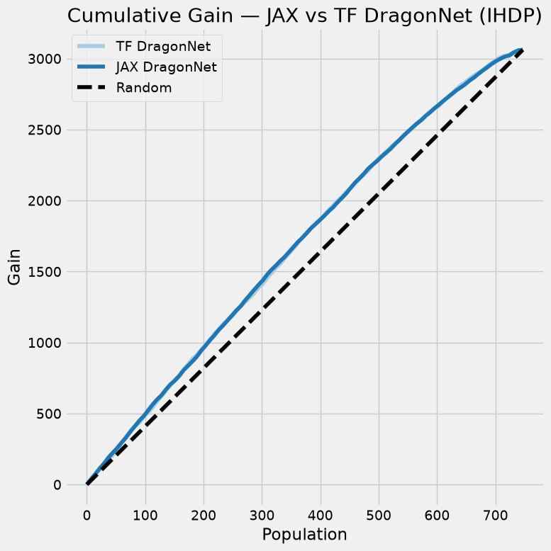
plot_gain(df_preds, outcome_col="y", treatment_col="w", treatment_effect_col="tau")
plt.title("Cumulative Gain — JAX vs TF DragonNet (IHDP)")
plt.tight_layout()
plt.show()

Note on training time: JAX train time includes one-time JIT compilation on the first mini-batch. TF time includes Keras graph building overhead. Both are measured end-to-end from fit() call to return.